Description of the WOMBATmid ocean biogeochemical model

        (\___/)  .-.   .-. .--. .-..-..---.  .--. .-----.
        / o o \  : :.-.: :: ,. :: '' :: .; :: .; :'-. .-'
       (   "   ) : :: :: :: :: :: .. ::   .':    :  : :
        \__ __/  : '' '' ;: :; :: :; :: .; :: :: :  : :
                  '.,'.,' '.__.':_;:_;:___.':_;:_;  :_;

 World Ocean Model of Biogeochemistry And Trophic-dynamics (WOMBAT)

Contact Pearse J. Buchanan and/or Dougal Squire for any questions
Pearse.Buchanan@csiro.au
Dougie.Squire@anu.edu.au

schematic

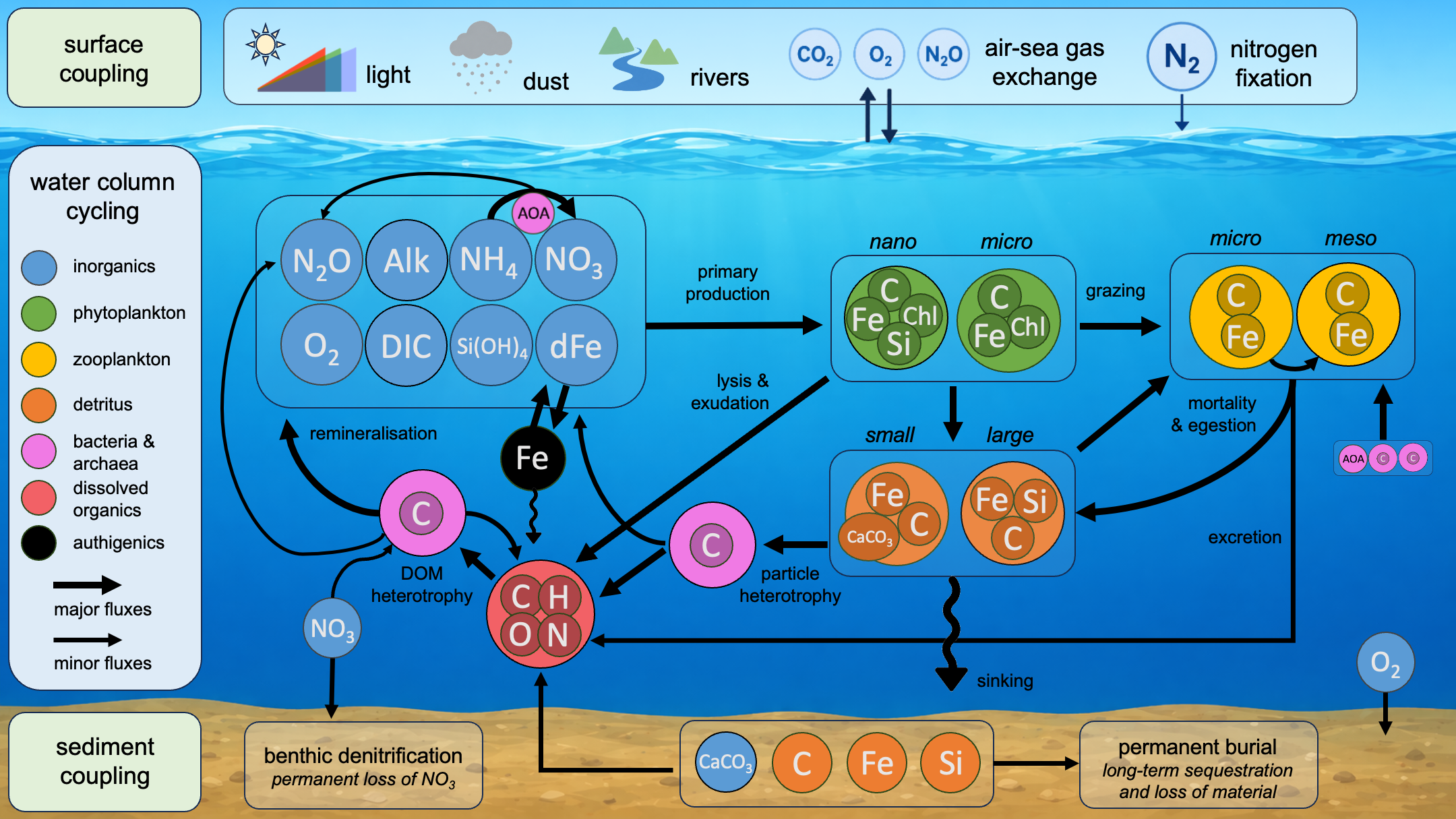
Executive summary

Currency of biomasses are in carbon units
Carbon chemistry uses the mocsy system by default (Orr & Epitalon, 2015)
Light is split into blue, green and red wavelengths and attenuated at rates dependent on ambient chlorophyll, organic particulate and inorganic particulate (CaCO₃) concentrations.
Nano- and Micro-phytoplankton perform photo-acclimation by altering their chlorophyll to carbon ratios according to the Geider, MacIntyre & Kana (1997) formulation.
Nano- and Micro-phytoplankton nutrient affinities for nitrogen, iron and silicic acid vary as a function of mean cell size via allometric relationships (Wickman et al. (2024)).
Nano- and Micro-phytoplankton prefer NH₄ over NO₃, but micro-phytoplankton have a growth advantage over nano-phytoplankton in high NO₃ conditions (Buchanan et al., 2025)
Nano- and Micro-phytoplankton growth is limited by an internal quota model for iron (Fe) (Droop, 1983) that responds to the cellular demands for nitrate reduction, respiration and chlorophyll, and represents luxury uptake.
Micro-phytoplankton growth is limited by an internal Si quota that gates division and varies Si:C ratios (Liu et al., 2016; Hutchins & Bruland 1998; Takeda 1998).
Nano- and Micro-phytoplankton exude dissolved organic matter in the form of carbohydrate (CH₂O) when under high light and nutrient limited conditions (Fogg, 1983; Hansell & Carlson, 2014).
The iron (Fe) cycle follows a combination of Aumont et al. (2015) and Tagliabue et al. (2023) to reflect varying Fe chemistry (solubility, ligand binding), scavenging and colloidal coagulation to sinking authigenic phases.
Biogenic silica (BSi) dissolution is informed by thermodynamics (Van Cappellen et al., 2002, temperature (Kamatani, 1982) and the activitiy of an implicit particle-associated heterotrophic bacteria (Bidle & Azam, 1999).
Micro- and Meso-zooplankton grazing assumes a Holling Type III functional form (Holling, 1959) and active switching between prey types (Gentleman et al., 2003).
Micro- and Meso-zooplankton routes Fe preferentially to egestion (i.e., faecal pellets) following Le Mézo & Galbraith (2021), enriching detritus in Fe.
Micro- and Meso-zooplankton dissolve CaCO₃ (Smith et al., 2024; White et al., 2018; Harris, 1994) but conserve biogenic silica due to acidic conditions in their gut (Dagg et al., 2003; Taucher et al., 2022).
The nitrogen cycle can be made to be open, with schemes for nitrogen fixation, anammox, and sedimentary denitrification that can be switched on or off at run time.
Nitrification of NH₄ to NO₃ is performed by an implicit population of ammonia oxidizing archaea.
Hydrolysation of particulate organic matter releases dissolved iron, ammonium and dissolved organic carbon, reflecting the preferential remineralisation of iron and nitrogen to inorganic forms before carbon.
CaCO₃ cycling is a function of the ambient seawater carbonate chemistry: production is affected by the substrate-inhibitor ratio (Lehmann & Bach, 2025); dissolution occurs in saturated waters ($\Omega$ > 1) due to reducing micro-environments and undersaturated waters ($\Omega$ < 1) (Kwon et al., 2024).
Sinking of small and large particulates is a function of mean radius, seawater dynamic viscosity and their excess density (Rubey, 1933). Radius varies via allometric scalings (e.g., Wickman et al., 2024), dynamic viscosity via thermohaline properties, and excess density by CaCO₃ and biogenic silica contents of the particles.
External sources of nitrate, DIC, alkalinity silicic acid and DOC via rivers.
Permanent burial of organics in sediments via Dunne et al. (2007).
External source of dissolved iron from aeolian deposition that includes mineral, fire and anthropogenic sources (Hamilton et al., 2020).
Major calibration and optimization of the model parameters... incoming.

Tracers

The following are the active tracers in WOMBAT-mid

#	Tracer	Code name	Description	Units	Default on?
1	O₂	`p_o2`	Dissolved oxygen	mol O2 kg^-1	Yes
2	NH₄	`p_nh4`	Ammonium	mol N kg^-1	Yes
3	NO₃	`p_no3`	Nitrate	mol N kg^-1	Yes
4	Si(OH)₄	`p_sil`	Silicic acid	mol Si kg^-1	Yes
5	dFe	`p_fe`	Dissolved iron	mol Fe kg^-1	Yes
6	Fe_sA	`p_safe`	Small sinking authigenic iron	mol Fe kg^-1	Yes
7	Fe_lA	`p_lafe`	Large sinking authigenic iron	mol Fe kg^-1	Yes
8	B_np^C	`p_phy`	Nano-phytoplankton	mol C kg^-1	Yes
9	B_mp^C	`p_dia`	Micro-phytoplankton	mol C kg^-1	Yes
10	B_mz^C	`p_zoo`	Micro-zooplankton	mol C kg^-1	Yes
11	B_Mz^C	`p_mes`	Meso-zooplankton	mol C kg^-1	Yes
12	B_sd^C	`p_sdet`	Small sinking detritus	mol C kg^-1	Yes
13	B_ld^C	`p_ldet`	Large sinking detritus	mol C kg^-1	Yes
14	B_np^Chl	`p_pchl`	Nano-phytoplankton chlorophyll content	mol C kg^-1	Yes
15	B_mp^Chl	`p_dchl`	Micro-phytoplankton chlorophyll content	mol C kg^-1	Yes
16	B_np^Fe	`p_phyfe`	Nano-phytoplankton iron content	mol Fe kg^-1	Yes
17	B_mp^Fe	`p_diafe`	Micro-phytoplankton iron content	mol Fe kg^-1	Yes
18	B_mp^Si	`p_diasi`	Micro-phytoplankton silicon content	mol Si kg^-1	Yes
19	B_mz^Fe	`p_zoofe`	Micro-zooplankton iron content	mol Fe kg^-1	Yes
20	B_Mz^Fe	`p_mesfe`	Meso-zooplankton iron content	mol Fe kg^-1	Yes
21	B_sd^Fe	`p_sdetfe`	Small sinking detritus iron content	mol Fe kg^-1	Yes
22	B_ld^Fe	`p_ldetfe`	Large sinking detritus iron content	mol Fe kg^-1	Yes
23	B_ld^Si	`p_ldetsi`	Large sinking detritus silicon content	mol Si kg^-1	Yes
24	B_DOM^C	`p_doc`	Dissolved organic carbon	mol C kg^-1	Yes
25	DIC	`p_dic`	Dissolved inorganic carbon	mol C kg^-1	Yes
26	Alk	`p_alk`	Dissolved alkalinity	mol Eq kg^-1	Yes
27	CaCO₃	`p_caco3`	Calcium carbonate	mol C kg^-1	Yes
28	DICp	no local	Preformed dissolved inorganic carbon	mol C kg^-1	No
29	DICr	`p_dicr`	Remineralised dissolved inorganic carbon	mol C kg^-1	No

Logical controls

The following are logical statements within the input.nml namelist file that can be switched to TRUE or FALSE at runtime.

Logical	Description	Default
`do_caco3_dynamics`	Production and dissolution of CaCO3 depends on carbon system state	.true.
`do_colloidal_shunt`	Fraction of dissolved iron is colloids that coagulate onto sinking material	.true.
`do_two_ligands`	Complex soluble iron using two ligands (weak + strong) rather than one	.false.
`do_burial`	Permanently bury a fraction of sinking detrital material into the sediments	.false.
`do_nitrogen_fixation`	Do implicit nitrogen fixation	.true.
`do_anammox`	Do implicit anaerobic ammonium oxidation	.true.
`do_benthic_denitrification`	Do implicit reduction of NO₃ in the sediment	.true.
`do_tracer_dicp`	Carry preformed dissolved inorganic carbon (dicp) as a tracer	.false.
`do_tracer_dicr`	Carry remineralised dissolved inorganic carbon (dicr) as a tracer	.false.
`do_viscous_sinking`	Rubey's formula uses a non-constant dynamic viscosity of seawater	.true.
`do_check_n_conserve`	Checks that the ecosystem calculations are conserving the mass of nitrogen	.false.
`do_check_c_conserve`	Checks that the ecosystem calculations are conserving the mass of carbon	.false.
`do_check_si_conserve`	Checks that the ecosystem calculations are conserving the mass of silicon	.false.
`do_check_fe_conserve`	Checks that the ecosystem calculations are conserving the mass of iron	.false.

We note that when do_two_ligands is set to .true., the ligK diagnostic variable reflects the binding strength of the strong ligand. However, when do_two_ligands is set to .false., this diagnostic (ligK) reflects the binding strength of the bulk ligand pool.

Diagnostic outputs

The following are all 2D diagnostic output variables from WOMBAT-mid.

Diagnostic	Description	Units
`pco2`	Surface aqueous partial pressure of CO₂	µatm
`npp2d`	Vertically integrated net primary production	mol C m^-2 s^-1
`rpp2d`	Vertically integrated regenerated primary production	mol C m^-2 s^-1
`zsp2d`	Vertically integrated zooplankton secondary production	mol C m^-2 s^-1
`sdet_radius`	Mean radius of small detrital particles	m
`ldet_radius`	Mean radius of large detrital particles	m
`det_sed_remin`	Rate of remineralisation of detritus in accumulated sediment	mol C m^-2 s^-1
`det_sed_depst`	Rate of deposition of detritus to sediment at base of water column	mol C m^-2 s^-1
`det_sed_denit`	Rate of benthic denitrification (removal of NO₃) in accumulated sediment	mol N m^-2 s^-1
`fbury`	Fraction of deposited detritus permanently buried beneath sediment	dimensionless
`ffebury`	Fraction of deposited iron permanently buried within sediment	dimensionless
`fdenit`	Fraction of sedimentary detritus remineralised via denitrification	dimensionless
`detfe_sed_remin`	Rate of remineralisation of detrital iron in accumulated sediment	mol Fe m^-2 s^-1
`detfe_sed_depst`	Rate of deposition of detrital iron to sediment at base of water column	mol Fe m^-2 s^-1
`detsi_sed_remin`	Rate of remineralisation of detrital silicon in accumulated sediment	mol Si m^-2 s^-1
`detsi_sed_depst`	Rate of deposition of detrital silicon to sediment at base of water column	mol Si m^-2 s^-1
`caco3_sed_remin`	Rate of remineralisation of CaCO₃ in accumulated sediment	mol C m^-2 s^-1
`caco3_sed_depst`	Rate of deposition of CaCO₃ to sediment at base of water column	mol C m^-2 s^-1
`zeuphot`	Depth of the euphotic zone (1% incident light)	m
`seddep`	Depth of the bottom layer	m
`sedmask`	Mask of active sediment points	dimensionless
`sedtemp`	Temperature in the bottom layer	°C
`sedsalt`	Salinity in the bottom layer	psu
`sedo2`	Oxygen concentration in the bottom layer	mol O₂ kg^-1
`sedno3`	Nitrate concentration in the bottom layer	mol N kg^-1
`sednh4`	Ammonium concentration in the bottom layer	mol N kg^-1
`sedsil`	Silicic acid concentration in the bottom layer	mol Si kg^-1
`seddic`	Dissolved inorganic carbon concentration in the bottom layer	mol C kg^-1
`sedalk`	Alkalinity concentration in the bottom layer	mol Eq kg^-1
`sedhtotal`	H⁺ ion concentration in the bottom layer	mol H⁺ kg^-1
`sedco3`	CO₃²⁻ ion concentration in the bottom layer	mol C kg^-1
`sedomega_cal`	Calcite saturation state in the bottom layer	dimensionless
`o2_stf`	Surface flux of dissolved oxygen into ocean	mol O2 m^-2 s^-1
`nh4_stf`	Surface flux of ammonium into ocean	mol N m^-2 s^-1
`no3_stf`	Surface flux of nitrate into ocean	mol N m^-2 s^-1
`sil_stf`	Surface flux of silicic acid into ocean	mol Si m^-2 s^-1
`fe_stf`	Surface flux of dissolved iron into ocean	mol Fe m^-2 s^-1
`sdet_stf`	Surface flux of small sinking detritus into ocean	mol C m^-2 s^-1
`ldet_stf`	Surface flux of large sinking detritus into ocean	mol C m^-2 s^-1
`doc_stf`	Surface flux of dissolved organic carbon into ocean	mol C m^-2 s^-1
`dic_stf`	Surface flux of dissolved inorganic carbon into ocean	mol C m^-2 s^-1
`dicp_stf`	Surface flux of preformed dissolved inorganic carbon into ocean	mol C m^-2 s^-1
`alk_stf`	Surface flux of alkalinity into ocean	mol Eq m^-2 s^-1
`no3_vstf`	Virtual flux of nitrate into ocean due to salinity restoring/correction	mol N m^-2 s^-1
`nh4_vstf`	Virtual flux of ammonium into ocean due to salinity restoring/correction	mol N m^-2 s^-1
`dic_vstf`	Virtual flux of dissolved inorganic carbon into ocean due to salinity restoring/correction	mol C m^-2 s^-1
`dicp_vstf`	Virtual flux of preformed dissolved inorganic carbon into ocean due to salinity restoring/correction	mol C m^-2 s^-1
`alk_vstf`	Virtual flux of alkalinity into ocean due to salinity restoring/correction	mol Eq m^-2 s^-1
`o2_btf`	Bottom flux of dissolved oxygen into ocean	mol O2 m^-2 s^-1
`no3_btf`	Bottom flux of nitrate into ocean	mol N m^-2 s^-1
`sil_btf`	Bottom flux of silicic acid into ocean	mol Si m^-2 s^-1
`doc_btf`	Bottom flux of dissolved organic carbon into ocean	mol C m^-2 s^-1
`fe_btf`	Bottom flux of dissolved iron into ocean	mol Fe m^-2 s^-1
`dic_btf`	Bottom flux of dissolved inorganic carbon into ocean	mol C m^-2 s^-1
`dicr_btf`	Bottom flux of remineralised dissolved inorganic carbon into ocean	mol C m^-2 s^-1
`alk_btf`	Bottom flux of alkalinity into ocean	mol Eq m^-2 s^-1

The following are all 3D diagnostic output variables from WOMBAT-mid.

Diagnostic	Description	Units
`htotal`	Concentration of H⁺ ion	mol H⁺ kg^-1
`omega_ara`	Saturation state of aragonite	dimensionless
`omega_cal`	Saturation state of calcite	dimensionless
`co3`	Carbonate ion concentration	mol C kg^-1
`co2_star`	CO2* (CO2(g) + H2CO3) concentration	mol C kg^-1
`dynvis_sw`	Seawater dynamic viscosity	kg m^-1 s^-1
`radbio`	Photosynthetically active radiation available for phytoplankton growth	W m^-2
`radmid`	Photosynthetically active radiation at centre point of grid cell	W m^-2
`radmld`	Photosynthetically active radiation averaged in mixed layer	W m^-2
`npp3d`	Net primary productivity	mol C kg^-1 s^-1
`rpp3d`	Regenerated primary productivity	mol C kg^-1 s^-1
`zsp3d`	Zooplankton secondary productivity	mol C kg^-1 s^-1
`phy_mumax`	Maximum growth rate of nano-phytoplankton	s^-1
`phy_mu`	Realised growth rate of nano-phytoplankton	s^-1
`pchl_mu`	Realised growth rate of nano-phytoplankton chlorophyll	mol C kg^-1 s^-1
`phy_lpar`	Limitation of nano-phytoplankton by light	dimensionless
`phy_kni`	Half-saturation coefficient of nitrogen uptake by nano-phytoplankton	mmol N m^-3
`phy_kfe`	Half-saturation coefficient of iron uptake by nano-phytoplankton	µmol Fe m^-3
`phy_lnit`	Limitation of nano-phytoplankton by nitrogen	dimensionless
`phy_lnh4`	Limitation of nano-phytoplankton by ammonium	dimensionless
`phy_lno3`	Limitation of nano-phytoplankton by nitrate	dimensionless
`phy_lfer`	Limitation of nano-phytoplankton by iron	dimensionless
`phy_dfeupt`	Uptake of dFe by nano-phytoplankton	mol Fe kg^-1 s^-1
`phy_feupreg`	Factor up regulation of dFe uptake by nano-phytoplankton	dimensionless
`phy_fedoreg`	Factor down regulation of dFe uptake by nano-phytoplankton	dimensionless
`phygrow`	Growth of nano-phytoplankton	mol C kg^-1 s^-1
`phydoc`	Overflow exudation of DOC by nano-phytoplankton	mol C kg^-1 s^-1
`phymorl`	Linear mortality of nano-phytoplankton	mol C kg^-1 s^-1
`phymorq`	Quadratic mortality of nano-phytoplankton	mol C kg^-1 s^-1
`dia_mumax`	Maximum growth rate of micro-phytoplankton	s^-1
`dia_mu`	Realised growth rate of micro-phytoplankton	s^-1
`dchl_mu`	Realised growth rate of micro-phytoplankton chlorophyll	mol C kg^-1 s^-1
`dia_lpar`	Limitation of micro-phytoplankton by light	dimensionless
`dia_kni`	Half-saturation coefficient of nitrogen uptake by micro-phytoplankton	mmol N m^-3
`dia_kfe`	Half-saturation coefficient of iron uptake by micro-phytoplankton	µmol Fe m^-3
`dia_ksi`	Half-saturation coefficient of silicic acid uptake by micro-phytoplankton	mmol Si m^-3
`dia_lnit`	Limitation of micro-phytoplankton by nitrogen	dimensionless
`dia_lnh4`	Limitation of micro-phytoplankton by ammonium	dimensionless
`dia_lno3`	Limitation of micro-phytoplankton by nitrate	dimensionless
`dia_lfer`	Limitation of micro-phytoplankton by iron	dimensionless
`dia_lsil`	Limitation of micro-phytoplankton by silicic acid	dimensionless
`dia_dfeupt`	Uptake of dFe by micro-phytoplankton	mol Fe kg^-1 s^-1
`dia_feupreg`	Factor up regulation of dFe uptake by micro-phytoplankton	dimensionless
`dia_fedoreg`	Factor down regulation of dFe uptake by micro-phytoplankton	dimensionless
`dia_silupt`	Uptake of silicic acid by micro-phytoplankton	mol Si kg^-1 s^-1
`dia_sidoreg`	Factor down regulation of silicic acid uptake by micro-phytoplankton	dimensionless
`diagrow`	Growth of micro-phytoplankton	mol C kg^-1 s^-1
`diadoc`	Overflow exudation of DOC by micro-phytoplankton	mol C kg^-1 s^-1
`diamorl`	Linear mortality of micro-phytoplankton	mol C kg^-1 s^-1
`diamorq`	Quadratic (density-dependent) mortality of micro-phytoplankton	mol C kg^-1 s^-1
`nitrfix`	Nitrogen fixation rate (NH₄ production)	mol N kg^-1 s^-1
`tri_lpar`	Limitation of implicit trichodesmium by light	dimensionless
`tri_lfer`	Limitation of implicit trichodesmium by iron	dimensionless
`trimumax`	Maximum growth rate of implicit trichodesmium	s^-1
`sileqc`	Equilibrium concentration of silicic acid	mol Si kg^-1
`disssi`	Dissolution rate of biogenic silica	s^-1
`bsidiss`	Dissolution of biogenic silica	mol Si kg^-1 s^-1
`feIII`	Free iron (Fe³⁺)	mol Fe kg^-1
`ligK`	Ligand stability constant	L mol^-1
`felig`	Ligand-bound dissolved iron	mol Fe kg^-1
`fecol`	Colloidal dissolved iron	mol Fe kg^-1
`fescasafe`	Scavenging of free Fe onto small authigenic particles due to smaller organics	mol Fe kg^-1 s^-1
`fescalafe`	Scavenging of free Fe onto large authigenic particles due to larger organics	mol Fe kg^-1 s^-1
`fecoag2safe`	Coagulation of colloidal dFe onto small authigenic particles	mol Fe kg^-1 s^-1
`fecoag2lafe`	Coagulation of colloidal dFe onto large authigenic particles	mol Fe kg^-1 s^-1
`safediss`	Dissolution of small colloidal authigenic Fe particles	mol Fe kg^-1 s^-1
`lafediss`	Dissolution of large colloidal authigenic Fe particles	mol Fe kg^-1 s^-1
`fesources`	Total source of dFe in water column	mol Fe kg^-1 s^-1
`fesinks`	Total sink of dFe in water column	mol Fe kg^-1 s^-1
`zooeps`	Micro-zooplankton community-wide prey capture rate coefficient	m⁶ mmolC^-2 s^-1
`zooprefphy`	Grazing dietary fraction of micro-zooplankton on nano-phytoplankton	mol C kg^-1 s^-1
`zooprefdia`	Grazing dietary fraction of micro-zooplankton on micro-phytoplankton	mol C kg^-1 s^-1
`zooprefsdet`	Grazing dietary fraction of micro-zooplankton on small detritus	mol C kg^-1 s^-1
`zoograzphy`	Grazing rate of micro-zooplankton on nano-phytoplankton	mol C kg^-1 s^-1
`zoograzdia`	Grazing rate of micro-zooplankton on micro-phytoplankton	mol C kg^-1 s^-1
`zoograzsdet`	Grazing rate of micro-zooplankton on small detritus	mol C kg^-1 s^-1
`zoomorl`	Linear mortality of micro-zooplankton	mol C kg^-1 s^-1
`zoomorq`	Quadratic (density-dependent) mortality of micro-zooplankton	mol C kg^-1 s^-1
`zooexcrphy`	Excretion rate of micro-zooplankton eating nano-phytoplankton	mol C kg^-1 s^-1
`zooexcrdia`	Excretion rate of micro-zooplankton eating micro-phytoplankton	mol C kg^-1 s^-1
`zooexcrsdet`	Excretion rate of micro-zooplankton eating small detritus	mol C kg^-1 s^-1
`zooegesphy`	Egestion rate of micro-zooplankton on nano-phytoplankton	mol C kg^-1 s^-1
`zooegesdia`	Egestion rate of micro-zooplankton on micro-phytoplankton	mol C kg^-1 s^-1
`zooegessdet`	Egestion rate of micro-zooplankton on small detritus	mol C kg^-1 s^-1
`meseps`	Meso-zooplankton community-wide prey capture rate coefficient	m⁶ mmolC^-2 s^-1
`mesprefphy`	Grazing dietary fraction of meso-zooplankton on nano-phytoplankton	mol C kg^-1 s^-1
`mesprefdia`	Grazing dietary fraction of meso-zooplankton on micro-phytoplankton	mol C kg^-1 s^-1
`mesprefsdet`	Grazing dietary fraction of meso-zooplankton on small detritus	mol C kg^-1 s^-1
`mesprefldet`	Grazing dietary fraction of meso-zooplankton on large detritus	mol C kg^-1 s^-1
`mesprefzoo`	Grazing dietary fraction of meso-zooplankton on micro-zooplankton	mol C kg^-1 s^-1
`mesgrazphy`	Grazing rate of meso-zooplankton on nano-phytoplankton	mol C kg^-1 s^-1
`mesgrazdia`	Grazing rate of meso-zooplankton on micro-phytoplankton	mol C kg^-1 s^-1
`mesgrazsdet`	Grazing rate of meso-zooplankton on small detritus	mol C kg^-1 s^-1
`mesgrazldet`	Grazing rate of meso-zooplankton on large detritus	mol C kg^-1 s^-1
`mesgrazzoo`	Grazing rate of meso-zooplankton on micro-zooplankton	mol C kg^-1 s^-1
`mesmorl`	Linear mortality of meso-zooplankton	mol C kg^-1 s^-1
`mesmorq`	Quadratic (density-dependent) mortality of meso-zooplankton	mol C kg^-1 s^-1
`mesexcrphy`	Excretion rate of meso-zooplankton eating nano-phytoplankton	mol C kg^-1 s^-1
`mesexcrdia`	Excretion rate of meso-zooplankton eating micro-phytoplankton	mol C kg^-1 s^-1
`mesexcrsdet`	Excretion rate of meso-zooplankton eating small detritus	mol C kg^-1 s^-1
`mesexcrldet`	Excretion rate of meso-zooplankton eating large detritus	mol C kg^-1 s^-1
`mesexcrzoo`	Excretion rate of meso-zooplankton eating micro-zooplankton	mol C kg^-1 s^-1
`mesegesphy`	Egestion rate of meso-zooplankton on nano-phytoplankton	mol C kg^-1 s^-1
`mesegesdia`	Egestion rate of meso-zooplankton on micro-phytoplankton	mol C kg^-1 s^-1
`mesegessdet`	Egestion rate of meso-zooplankton on small detritus	mol C kg^-1 s^-1
`mesegesldet`	Egestion rate of meso-zooplankton on large detritus	mol C kg^-1 s^-1
`mesegeszoo`	Egestion rate of meso-zooplankton on micro-zooplankton	mol C kg^-1 s^-1
`reminrpoc`	Rate of hydrolysation of particulate organic matter	s^-1
`reminrdoc`	Rate of remineralisation of dissolved organic matter	s^-1
`sdetremi`	Hydrolysation of small sinking detritus	mol C kg^-1 s^-1
`ldetremi`	Hydrolysation of large sinking detritus	mol C kg^-1 s^-1
`docremi`	Remineralisation of dissolved organic carbon	mol C kg^-1 s^-1
`ammox`	Ammonia oxidation rate (NH₄ consumption)	mol N kg^-1 s^-1
`aoa_loxy`	Limitation of ammonia oxidation by oxygen	dimensionless
`aoa_lnh4`	Limitation of ammonia oxidation by ammonium	dimensionless
`aoa_mu`	Realized growth rate of ammonia oxidizing archaea	s^-1
`anammox`	Anammox rate (NH₄ consumption)	mol kg^-1 s^-1
`aox_lnh4`	Limitation of anammox bacteria by ammonium	dimensionless
`aox_mu`	Realized growth rate of anammox bacteria	s^-1
`pic2poc`	Inorganic (CaCO3) to organic carbon ratio	dimensionless
`dissratcal`	Dissolution rate of calcite CaCO3	s^-1
`dissratara`	Dissolution rate of aragonite CaCO3	s^-1
`dissratpoc`	Dissolution rate of CaCO3 due to POC (detritus) remineralization	s^-1
`zoodiss`	Dissolution of CaCO3 due to micro-zooplankton grazing	mol CaCO3 kg^-1 s^-1
`mesdiss`	Dissolution of CaCO3 due to meso-zooplankton grazing	mol CaCO3 kg^-1 s^-1
`caldiss`	Dissolution of calcite CaCO3	mol CaCO3 kg^-1 s^-1
`aradiss`	Dissolution of aragonite CaCO3	mol CaCO3 kg^-1 s^-1
`pocdiss`	Dissolution of CaCO3 due to POC remin	mol CaCO3 kg^-1 s^-1
`sdet_density`	Mean density of small detrital particles	kg m^-3
`ldet_density`	Mean density of large detrital particles	kg m^-3
`sdet_vmove`	Sinking rate of small detritus	m s^-1
`sdetfe_vmove`	Sinking rate of small detrital iron	m s^-1
`ldet_vmove`	Sinking rate of large detritus	m s^-1
`ldetfe_vmove`	Sinking rate of large detrital iron	m s^-1
`ldetsi_vmove`	Sinking rate of large detrital silicon	m s^-1
`caco3_vmove`	Sinking rate of CaCO3	m s^-1

Subroutine - "update_from_source"

The subroutine generic_WOMBATmid_update_from_source is the heart of the World Ocean Model of Biogeochemistry And Trophic‑dynamics (WOMBAT). Its purpose is to apply biological source–sink terms to ocean tracers (nutrients, phytoplankton, zooplankton, particulate detritus, dissolved and particulate iron, dissolved organics carbon, alkalinity, oxygen and carbon pools) at each time‑step. The subroutine is documented internally by a list of numbered steps (see code comments). These steps are:

Light attenuation through the water column.
Nutrient limitation of phytoplankton.
Temperature-dependent metabolism and POC-->DOC.
Light limitation of phytoplankton.
Realized growth rate of phytoplankton.
Dissolved organic carbon release by phytoplankton.
Synthesis of chlorophyll.
Phytoplankton uptake of iron.
Phytoplankton uptake of silicic acid.
Iron chemistry (scavenging, coagulation, dissolution).
Biogenic silica dissolution.
Mortality terms.
Zooplankton grazing, egestion, excretion and assimilation.
Implicit nitrogen fixation.
Calcium carbonate production and dissolution.
Chemoautotrophy.
Tracer tendencies.
Check for conservation of mass.
Additional operations on tracers.
Sinking rate of particulates.
Sedimentary processes.

Below is a step‑by‑step explanation of each section together with the key equations. Variable names in grey follow the Fortran code, while variable names in $math font$ are pointers to the equations; i,j,k refer to horizontal and vertical indices; [square brackets] denote units. If a variable is without i,j,k dimensions, this variable is held as a scalar and not an array.

The model carries tracers in [mol kg-1]. That is, moles of solute/tracer per kilogram of seawater (i.e., molality). Some calculations herein are performed by converting tracers to units of [mmol m-3] or in the case of dissolved iron [µmol m-3]. However, we stress that all tracer tendency terms are converted back to [mol kg-1 s-1] when sources and sinks are applied.

Parameter set and default values

Parameter	Description	Value	Units
`alphabio_phy`	Initial slope of P–I curve (nano-phytoplankton)	1.5	mol C (mol Chl)^-1 (W m^-2)^-1
`abioa_phy`	Max growth rate parameter a (nano-phytoplankton)	0.7/86400.0	s^-1
`bbioa_phy`	Max growth rate parameter b (nano-phytoplankton) (Q10 = b^(10))	1.055	dimensionless
`phyprefnh4`	NH₄ preference over NO₃ (nano-phytoplankton)	5.0	dimensionless
`phykn`	Half-saturation coefficient N uptake (nano-phytoplankton)	1.0	mmol N m^-3
`phykf`	Half-saturation coefficient Fe uptake (nano-phytoplankton)	1.0	µmol Fe m^-3
`phyminqc`	Min Chl:C (nano-phytoplankton)	0.008	mol Chl (mol C)^-1
`phymaxqc`	Max Chl:C (nano-phytoplankton)	0.065	mol Chl (mol C)^-1
`phyoptqf`	Optimal Fe:C (nano-phytoplankton)	10e-6	mol Fe (mol C)^-1
`phymaxqf`	Max Fe:C (nano-phytoplankton)	50e-6	mol Fe (mol C)^-1
`phylmor`	Linear mortality rate (nano-phytoplankton)	0.001/86400.0	s^-1
`phyqmor`	Quadratic mortality rate (nano-phytoplankton)	0.05/86400.0	(mmol C m^-3)^-1 s^-1
`phybiot`	Biomass threshold (nano-phytoplankton)	1.0	mmol C m^-3
`alphabio_dia`	Initial slope of P–I curve (micro-phytoplankton)	2.5	mol C (mol Chl)^-1 (W m^-2)^-1
`abioa_dia`	Max growth rate parameter a (micro-phytoplankton)	1.0/86400.0	s^-1
`bbioa_dia`	Max growth rate parameter b (micro-phytoplankton) (Q10 = b^(10))	1.070	dimensionless
`diaprefnh4`	NH₄ preference over NO₃ (micro-phytoplankton)	5.0	dimensionless
`diakn`	Half-saturation coefficient N uptake (micro-phytoplankton)	2.4	mmol N m^-3
`diakf`	Half-saturation coefficient Fe uptake (micro-phytoplankton)	2.7	µmol Fe m^-3
`diaks`	Half-saturation coefficient Si uptake (micro-phytoplankton)	6.7	mmol Si m^-3
`diaminqc`	Min Chl:C (micro-phytoplankton)	0.004	mol Chl (mol C)^-1
`diamaxqc`	Max Chl:C (micro-phytoplankton)	0.060	mol Chl (mol C)^-1
`diaoptqf`	Optimal Fe:C (micro-phytoplankton)	10e-6	mol Fe (mol C)^-1
`diamaxqf`	Max Fe:C (micro-phytoplankton)	65e-6	mol Fe (mol C)^-1
`diaminqs`	Min Si:C (micro-phytoplankton)	0.04	mol Si (mol C)^-1
`diaoptqs`	Optimal Si:C (micro-phytoplankton)	0.13	mol Si (mol C)^-1
`diamaxqs`	Max Si:C (micro-phytoplankton)	0.60	mol Si (mol C)^-1
`diaVmaxs`	Max Si uptake (micro-phytoplankton)	0.1/86400.0	mol Si (mol C)^-1 s^-1
`dialmor`	Linear mortality rate (micro-phytoplankton)	0.001/86400.0	s^-1
`diaqmor`	Quadratic mortality rate (micro-phytoplankton)	0.05/86400.0	(mmol C m^-3)^-1 s^-1
`diabiot`	Biomass threshold (micro-phytoplankton)	0.5	mmol C m^-3
`alphabio_tri`	Initial slope of P–I curve (trichodesmium)	1.8	mol C (mol Chl)^-1 (W m^-2)^-1
`trikf`	Fe half-saturation coefficient (trichodesmium)	0.125	µmol Fe m^-3
`trichlc`	Chl:C (trichodesmium)	0.01	mol Chl (mol C)^-1
`trin2c`	N:C (trichodesmium)	50/300	mol N (mol C)^-1
`chltau`	Chlorophyll adjustment timescale	86400	s
`overflow`	Max DOC exudation fraction by phytoplankton	0.50	dimensionless
`bbioh`	Heterotrophic growth scaling parameter b (Q10 = b^(10))	1.072	dimensionless
`zooCingest`	Micro-zooplankton C ingestion efficiency	0.70	mol C (mol C)^-1
`zooCassim`	Micro-zooplankton C assimilation efficiency	0.40	mol C (mol C)^-1
`zooFeingest`	Micro-zooplankton Fe ingestion efficiency	0.06	mol Fe (mol Fe)^-1
`zooFeassim`	Micro-zooplankton Fe assimilation efficiency	0.60	mol Fe (mol Fe)^-1
`zooexcrdom`	Micro-zooplankton excretion fraction routed to DOM	0.70	dimensionless
`zoogmax`	Micro-zooplankton max grazing rate	3.3/86400.0	s^-1
`zooepsphy`	Micro-zooplankton prey capture efficiency (nano-phytoplankton)	0.40/86400.0	m⁶ mmol^-2 s^-1
`zooepsdia`	Micro-zooplankton prey capture efficiency (micro-phytoplankton)	0.40/86400.0	m⁶ mmol^-2 s^-1
`zooepssdet`	Micro-zooplankton prey capture efficiency (small detritus)	0.40/86400.0	m⁶ mmol^-2 s^-1
`zprefphy`	Micro-zooplankton preference (nano-phytoplankton)	1.0	dimensionless
`zprefdia`	Micro-zooplankton preference (micro-phytoplankton)	0.25	dimensionless
`zprefsdet`	Micro-zooplankton preference (small detritus)	1.0	dimensionless
`zoolmor`	Micro-zooplankton linear mortality rate	0.002/86400.0	s^-1
`zooqmor`	Micro-zooplankton quadratic mortality rate	0.05/86400.0	(mmol C m^-3)^-1 s^-1
`zoopreyswitch`	Micro-zooplankton prey switching exponent	1.8	dimensionless
`mesCingest`	Meso-zooplankton C ingestion	0.75	mol C (mol C)^-1
`mesCassim`	Meso-zooplankton C assimilation	0.50	mol C (mol C)^-1
`mesFeingest`	Meso-zooplankton Fe ingestion	0.43	mol Fe (mol Fe)^-1
`mesFeassim`	Meso-zooplankton Fe assimilation	0.75	mol Fe (mol Fe)^-1
`mesexcrdom`	Meso-zooplankton excretion fraction routed to DOM	0.35	dimensionless
`mesgmax`	Meso-zooplankton maximum grazing rate	0.30/86400.0	s^-1
`mesepsphy`	Meso-zooplankton prey capture efficiency (nano-phytoplankton)	0.11/86400.0	m⁶ mmol^-2 s^-1
`mesepsdia`	Meso-zooplankton prey capture efficiency (micro-phytoplankton)	0.20/86400.0	m⁶ mmol^-2 s^-1
`mesepssdet`	Meso-zooplankton prey capture efficiency (small detritus)	0.05/86400.0	m⁶ mmol^-2 s^-1
`mesepsldet`	Meso-zooplankton prey capture efficiency (large detritus)	0.10/86400.0	m⁶ mmol^-2 s^-1
`mesepszoo`	Meso-zooplankton prey capture efficiency (micro-zooplankton)	0.10/86400.0	m⁶ mmol^-2 s^-1
`mprefphy`	Meso-zooplankton preference (nano-phytoplankton)	0.5	dimensionless
`mprefdia`	Meso-zooplankton preference (micro-phytoplankton)	1.0	dimensionless
`mprefsdet`	Meso-zooplankton preference (small detritus)	1.0	dimensionless
`mprefldet`	Meso-zooplankton preference (large detritus)	1.0	dimensionless
`mprefzoo`	Meso-zooplankton preference (micro-zooplankton)	1.0	dimensionless
`meslmor`	Meso-zooplankton linear mortality rate	0.002/86400.0	s^-1
`mesqmor`	Meso-zooplankton quadratic mortality rate	0.75/86400.0	(mmol C m^-3)^-1 s^-1
`mespreyswitch`	Meso-zooplankton prey switching exponent	1.8	dimensionless
`detqrem`	Detritus hydrolysation rate	0.7/86400.0	(mmol C m^-3)^-1 s^-1
`docqrem`	Dissolved organic matter remineralisation rate	0.2/86400.0	(mmol C m^-3)^-1 s^-1
`detlrem_sed`	Sediment detritus hydrolysation rate	0.005/86400.0	s^-1
`sdetphi`	Porosity (small detritus)	0.25	dimensionless
`ldetphi`	Porosity (large detritus)	0.75	dimensionless
`detrho`	Detritus density	1375	kg m^-3
`caco3rho`	CaCO3 density	2710	kg m^-3
`bsirho`	Opal density	2000	kg m^-3
`phyrad0`	Nano-phytoplankton mean radius	10	µm
`diarad0`	Micro-phytoplankton mean radius	50	µm
`zoorad0`	Micro-zooplankton mean radius	30	µm
`mesrad0`	Meso-zooplankton mean radius	1000	µm
`caco3lrem`	CaCO₃ dissolution rate	0.01/86400.0	s^-1
`caco3lrem_sed`	Sediment CaCO₃ dissolution rate	0.01/86400.0	s^-1
`f_inorg`	Base inorganic fraction (PIC:POC ratio)	0.04	mol CaCO3 (mol C)^-1
`disscal`	Calcite dissolution rate	0.10/86400.0	s^-1
`dissara`	Aragonite dissolution rate	0.10/86400.0	s^-1
`dissdet`	Fraction CaCO3 dissolved per detritus hydrolyzed	0.20	mol CaCO3 (mol C)^-1
`fgutdiss`	Zooplankton gut CaCO3 dissolution efficiency	0.80	dimensionless
`ligW`	Weak ligand concentration	1.7	µmol m^-3
`ligS`	Strong ligand concentration	0.4	µmol m^-3
`dfefloor`	Minimum open water concentration of dissolved iron (detection limit)	0.025	µmol Fe m^-3
`detfesedfloor`	Minimum detrital iron sediment reservoir in shallow (≤200m) columns	30.0	µmol Fe m^-2
`kscav_dfe`	Free dissolved iron scavenging rate	0.01/86400.0	(mmol mass of particle m^-3)^-1 s^-1
`kcoag_dfe`	Colloidal dissolved iron coagulation rate	1e-5/86400.0	(mmol C m^-3)^-1 s^-1
`kagg_col`	Colloidal dissolved iron aggregation rate	0.1/86400.0	s^-1
`kagg_kcol`	Half-saturation coefficient for colloidal iron aggregation	2.0	µmol Fe m^-3
`ksafe_dfe`	Authigenic iron dissolution rate (small)	1e-4/86400	s^-1
`klafe_dfe`	Authigenic iron dissolution rate (large)	1e-4/86400	s^-1
`wsafe`	Authigenic iron sinking rate (small)	0.5/86400	m s^-1
`wlafe`	Authigenic iron sinking rate (large)	5.0/86400	m s^-1
`bsi_alpha`	Natural-log intercept of temperature-dependent biogenic silica dissolution	-10	ln(per hour)
`bsi_fbac`	Bacterial enhancement factor for silica dissolution	10	dimensionless
`bsi_kbac`	Half-saturation coefficient for bacterial enhancement of silica dissolution	0.5	mmol C m^-3
`bsilrem_sed`	Base sediment biogenic silica dissolution rate	2.8e-8	s^-1
`aoa_knh4`	AOA NH₄ half-saturation coefficient	0.1	mmol N m^-3
`aoa_poxy`	AOA O₂ diffusive uptake limit	275/86400	(mmol C biomass m³)^-1 s^-1
`aoa_ynh4`	AOA NH₄ demand per C biomass	11.0	mol N (mol C)^-1
`aoa_yoxy`	AOA O₂ demand per C biomass	15.5	mol O₂ (mol C)^-1
`aoxkn`	Anammox NH₄ half-saturation coefficient	0.5	mmol N m^-3
`aoxmumax`	Anammox maximum growth rate	0.0025/86400	s^-1
`bottom_thickness`	Bottom layer thickness	0.1	m

1. Light attenuation through the water column.

Photosynthetically available radiation (PAR) is split into blue, green and red wavelengths. The incoming visible (photosynthetically available) short wave radiation flux (PAR, [W m^-2]) is received from the physical model, and is then split evenly into each of blue, green and red light bands.

At the top (par_bgr_top(k,b), $PAR^{top}$) and mid‑point (par_bgr_mid(k,b), $PAR^{mid}$) of each layer k we calculate the downward irradiance by exponential decay of each band b through the layer thickness (dzt(i,j,k), $\Delta z$, [m]) using band‑specific attenuation coefficients. These attenuation coefficients are related to the concentration of chlorophyll (chl, [mg m^-3]), organic detritus (ndet, [mg N m^-3]) and calcium carbonate (carb, [kg m^-3]) in the water column.

For chlorophyll, attenuation coefficients for each of blue, green and red light (zbgr(ichl,b), [m^-1]) are retrieved from the look-up table of Morel & Maritorena (2001) (their Table 2) that explicitly relates chlorophyll concentration to attenuation rates and accounts for the packaging effect of chlorophyll in larger cells. Within zbgr(ichl,b), ichl is an integer that corresponds to a particular band of chlorophyll concentration, with increasing chlorophyll concentrations associated with increasing attenuation.

For organic detritus, attenuation coefficients for blue, green and red light (dbgr(b), [(mg N m^-3)^-1 m^-1]) are taken from Dutkiewicz et al. (2015) (their Fig. 1b), while for calcium carbonate (cbgr(b), [(kg CaCO₃ m^-3)^-1m^-1]) we take the coefficients defined in Soja-Wozniak et al. (2019). For both detritus and calcium carbonate, these studies provide concentration-normalized attenuation coefficients, which must be multiplied against concentrations to retrieve the correct units of [m^-1].

Because WOMBAT-mid has two forms of phytoplankton (nanophytoplankton and microphytoplankton) with their own chlorophyll quotas and two forms of particulate detritus (small and large), we sum both chlorophyll pools and particulate detritus pools to return the total chlorophyll and the total particulate detritus.

As an example, the PAR in the blue band (b=1) at the top of level k is computed as

\[ \begin{align} PAR^{top}(k,1) =& \quad PAR^{top}(k-1,1) * e^{(-ex_{bgr}(k-1,1) * \Delta z(k-1))} \end{align} \]

where the total attenutation rate of blue light in the grid cell above k is the sum of attenuation due to all particulates in that grid cell, which includes chlorophyll, detritus and calcium carbonate:

\[ \begin{align} ex_{bgr}(k-1,1) =& \quad ex_{chl}(k-1,1) + ex_{det}(k-1,1) + ex_{CaCO_3}(k-1,1) \end{align} \]

where
- $ex_{chl}(k-1,1)$ is the attenuation rate of blue light (b=1) in the overlying grid cell (k-1) due to chlorophyll (zbgr(2,ichl), [m^-1])
- $ex_{det}(k-1,1)$ is the attenuation rate of blue light (b=1) in the overlying grid cell (k-1) due to detritus (ndet * dbgr(1), [m^-1])
- $ex_{CaCO_3}(k-1,1)$ is the attenuation rate of blue light (b=1) in the overlying grid cell (k-1) due to calcium carbonate (carb * cbgr(1), [m^-1])

The irradiance in the red band (b=3) at the mid point of layer k, in contrast, is equal to

\[ \begin{align} PAR^{mid}(k,3) =& \quad PAR^{mid}(k-1,3) * e^{(-0.5*(ex_{bgr}(k-1,3) * \Delta z(k-1) + ex_{bgr}(k,3) * \Delta z(k)))} \end{align} \]

where
- $PAR^{mid}(k-1,3)$ is the red light (b=3) at the mid-point of the overlying grid cell (par_bgr_mid(k-1,3), [W m^-2])
- $ex_{bgr}(k-1,3)$ is the total attenuation of red light (b=3) in the overlying grid cell (ek_bgr(k-1,3), [m^-1])
- $ex_{bgr}(k,3)$ is the total attenuation of red light (b=3) in the current grid cell (ek_bgr(k,3), [m^-1])
- $\Delta z(k-1)$ and $\Delta z(k)$ are the grid cell thicknesses of the overlying and current grid cells (dzt(i,j,k), [m])

The total PAR available to phytoplantkon is assumed to be the sum of the blue, green and red bands. Because we assume that phytoplankton are homogenously distributed within a layer k, but we do not assume that light is homogenously distributed within that layer, we solve for the PAR that is seen by the average phytoplankton within that cell (radbio, $PAR$, [W m^-2])

\[ \begin{align} PAR(k) =& \quad \sum_{b=1}^3 \dfrac{(PAR^{top}(k,b) - PAR^{top}(k+1,b))}{ex_{bgr}(k,b) * \Delta z(k)} \end{align} \]

where
- $PAR^{top}(k,b)$ is the incoming photosynthetically active radiation at the top of grid cell k and light band b (par_bgr_top(k,b), [W m^-2])
- $ex_{bgr}(k,b)$ is the attenuation rate of light band b in grid cell k (ek_bgr(k,b), [m^-1])
- $\Delta z(k)$ is the grid cell thickness of grid cell k (dzt(i,j,k), [m])

This ensures phytoplankton growth in the model responds to the mean light they experience in the cell, not just light at one point. See Eq. 19 from Baird et al. (2020).

The euphotic depth (zeuphot(i,j), [m]) is defined as the depth where radbio falls below the 1% threshold of incidient shortwave radiation or below 0.01 W m^-2, whichever is shallower.

2. Nutrient limitation of phytoplankton.

At the start of each vertical loop k=1 through k=kmax the code computes the biomass of nano-phytoplankton (phy_mmolm3, $B_{np}$, [mmol C m^-3]) and micro-phytoplankton (dia_mmolm3, $B_{mp}$, [mmol C m^-3]). Phytoplankton biomass is used to scale how nitrogen in the form of nitrate (no3_mmolm3, NO₃, [mmol N m^-3]) and ammonium (nh4_mmolm3, NH₄, [mmol N m^-3]), dissolved iron (fe_umolm3, $dFe$, [µmol dFe m^-3]) and silicic acid in the case of micro-phytoplankton (sil_mmolm3, H₄SiO₄, [mmol Si m^-3]) affect the growth of phytoplankton. Using compilations of marine phytoplankton and zooplankton communities, Wickman et al. (2024) show that the nutrient affinity, $aff$, of a phytoplankton cell is related to its volume, $V$, via

\[ \begin{align} aff =& \quad V^{-0.57} \end{align} \]

Additionally, the authors demonstrate that the volume of the average phytoplankton cell is related to the density (i.e., concentration) of phytoplankton via

\[ \begin{align} V =& \quad (B_{phy})^{0.65} \end{align} \]

when combining panels c and f of their Figure 1. This then relates the affinity of an average cell to the concentration of phytoplankton biomass as

\[ \begin{align} aff =& \quad (B_{phy})^{-0.37} \end{align} \]

With this information, we allow the half-saturation terms for nitrogen (phy_kni(i,j,k), $K_{np}^{N}$, [mmol N m^-3]; dia_kni(i,j,k), $K_{mp}^{N}$, [mmol N m^-3]), dissolved iron (phy_kfe(i,j,k), $K_{np}^{Fe}$, [µmol dFe m^-3]; dia_kfe(i,j,k), $K_{mp}^{Fe}$, [µmol dFe m^-3]) and silicic acid (dia_ksi(i,j,k), $K_{mp}^{Si}$, [mmol Si m^-3]) uptake to vary as a function of phytoplankton biomass concentration. We set reference values for the half-saturation coefficient of nitrogen (phykn, $K_{np}^{N,0}$, [mmol N m^-3]; diakn, $K_{mp}^{N,0}$, [mmol N m^-3]), dissolved iron (phykf, $K_{np}^{Fe,0}$, [µmol dFe m^-3]; diakf, $K_{mp}^{Fe,0}$, [µmol dFe m^-3]) and silicic acid (diaks, $K_{mp}^{Si,0}$, [mmol Si m^-3]) as input parameters to the model, and also set thresholds of nano-phytoplankton concentration (phybiot, $B_{np}^{thresh}$, [mmol C m^-3]) and micro-phytoplankton concentration (diabiot, $B_{mp}^{thresh}$, [mmol C m^-3]) beneath which cell size cannot decrease and affinity can no longer increase. At this minimum, where affinity is maximised, the half-saturation coefficients are bounded to be 10% of their reference values.

\[ \begin{align} K_{np}^{N} =& \quad K_{np}^{N,0} * \max(0.1, \max(0.0, (B_{np}-B_{np}^{thresh}))^{0.37} ) \\ K_{np}^{Fe} =& \quad K_{np}^{Fe,0} * \max(0.1, \max(0.0, (B_{np}-B_{np}^{thresh}))^{0.37} ) \\ K_{mp}^{N} =& \quad K_{mp}^{N,0} * \max(0.1, \max(0.0, (B_{mp}-B_{mp}^{thresh}))^{0.37} ) \\ K_{mp}^{Fe} =& \quad K_{mp}^{Fe,0} * \max(0.1, \max(0.0, (B_{mp}-B_{mp}^{thresh}))^{0.37} ) \\ K_{mp}^{Si} =& \quad K_{mp}^{Si,0} * \max(0.1, \max(0.0, (B_{mp}-B_{mp}^{thresh}))^{0.37} ) \end{align} \]

where
- $K_{np}^{N}$ and $K_{mp}^{N}$ are the half-saturation coefficients for nitrogen uptake by nano- and micro-phytoplankton (phy_kni(i,j,k) and dia_kni(i,j,k), [mmol N m^-3])
- $K_{np}^{Fe}$ and $K_{mp}^{Fe}$ are the half-saturation coefficients for iron uptake by nano- and micro-phytoplankton (phy_kfe(i,j,k) and dia_kfe(i,j,k), [µmol Fe m^-3])
- $K_{mp}^{Si}$ is the half-saturation coefficient of silicic acid uptake by micro-phytoplankton (dia_ksi(i,j,k), [mmol Si m^-3])

Limitation of phytoplankton growth by nitrogen (phy_lnit(i,j,k), $L_{np}^{N}$), [dimensionless]; dia_lnit(i,j,k), $L_{mp}^{N}$), [dimensionless]) is split between ammonium (phy_lnh4(i,j,k), $L_{np}^{NH_4}$), [dimensionless]; dia_lnh4(i,j,k), $L_{mp}^{NH_4}$), [dimensionless]) and nitrate (phy_lno3(i,j,k), $L_{np}^{NO_3}$), [dimensionless]; dia_lno3(i,j,k), $L_{mp}^{NO_3}$), [dimensionless]). Phytoplankton preferentially consume and grow on ammonium because it is most efficiently converted to glutamate for biomass synthesis, while nitrate must be first reduced within the cell (Dortch, 1990). To represent this preference, we follow Buchanan et al., 2025 who assert a 5-fold preference of phytoplankton for ammonium over nitrate and show that this reproduces preferences of ammonium-fueled growth in ocean field data.

\[ \begin{align} l_{np}^{NH_4} =& \quad \dfrac{NH_4}{NH_4 + K_{np}^{N}} \\ l_{np}^{NO_3} =& \quad \dfrac{NO_3}{NO_3 + K_{np}^{N}} \\ l_{np}^{N} =& \quad \dfrac{NH_4 + NO_3}{NH_4 + NO_3 + K_{np}^{N}} \\ L_{np}^{NH_4} =& \quad \dfrac{5 \cdot l_{np}^{N} l_{np}^{NH_4}}{l_{np}^{NO_3} + 5 \cdot l_{np}^{NH_4}} \\ L_{np}^{NO_3} =& \quad \dfrac{l_{np}^{N} l_{np}^{NO_3}}{l_{np}^{NO_3} + 5 \cdot l_{np}^{NH_4}} \\ L_{np}^{N} =& \quad L_{np}^{NH_4} + L_{np}^{NO_3} \end{align} \]

where
- NH₄ is the in situ concentration of ammonium (nh4_mmolm3, [mmol N m^-3])
- NO₃ is the in situ concentration of nitrate (no3_mmolm3, [mmol N m^-3])
- $l_{np}^{NH_4}$ is the limitation term of nano-phytoplankton growth on ammonium before preferencing (phy_limnh4, [dimensionless])
- $l_{np}^{NO_3}$ is the limitation term of nano-phytoplankton growth on nitrate before preferencing (phy_limno3, [dimensionless])
- $l_{np}^{N}$ is the limitation term of nano-phytoplankton growth on nitrogen before preferencing (phy_limdin, [dimensionless])
- $L_{np}^{NH_4}$ is the limitation term of nano-phytoplankton growth on ammonium (phy_lnh4(i,j,k), [dimensionless])
- $L_{np}^{NO_3}$ is the limitation term of nano-phytoplankton growth on nitrate (phy_lno3(i,j,k), [dimensionless])
- $L_{np}^{N}$ is the limitation term of nano-phytoplankton growth on nitrogen (phy_lnit(i,j,k), [dimensionless])

The same set of equations are applied to micro-phytoplankton:

\[ \begin{align} l_{mp}^{NH_4} =& \quad \dfrac{NH_4}{NH_4 + K_{mp}^{N}} \\ l_{mp}^{NO_3} =& \quad \dfrac{NO_3}{NO_3 + K_{mp}^{N}} \\ l_{mp}^{N} =& \quad \dfrac{NH_4 + NO_3}{NH_4 + NO_3 + K_{mp}^{N}} \\ L_{mp}^{NH_4} =& \quad \dfrac{5 \cdot l_{mp}^{N} l_{mp}^{NH_4}}{l_{mp}^{NO_3} + 5 \cdot l_{mp}^{NH_4}} \\ L_{mp}^{NO_3} =& \quad \dfrac{l_{mp}^{N} l_{mp}^{NO_3}}{l_{mp}^{NO_3} + 5 \cdot l_{mp}^{NH_4}} \\ L_{mp}^{N} =& \quad L_{mp}^{NH_4} + L_{mp}^{NO_3} \end{align} \]

where
- NH₄ is the in situ concentration of ammonium (nh4_mmolm3, [mmol N m^-3])
- NO₃ is the in situ concentration of nitrate (no3_mmolm3, [mmol N m^-3])
- $l_{mp}^{NH_4}$ is the limitation term of micro-phytoplankton growth on ammonium before preferencing (dia_limnh4, [dimensionless])
- $l_{mp}^{NO_3}$ is the limitation term of micro-phytoplankton growth on nitrate before preferencing (dia_limno3, [dimensionless])
- $l_{mp}^{N}$ is the limitation term of micro-phytoplankton growth on nitrogen before preferencing (dia_limdin, [dimensionless])
- $L_{mp}^{NH_4}$ is the limitation term of micro-phytoplankton growth on ammonium (dia_lnh4(i,j,k), [dimensionless])
- $L_{mp}^{NO_3}$ is the limitation term of micro-phytoplankton growth on nitrate (dia_lno3(i,j,k), [dimensionless])
- $L_{mp}^{N}$ is the limitation term of micro-phytoplankton growth on nitrogen (dia_lnit(i,j,k), [dimensionless])

Note that although phytoplankton prefer NH₄ over NO₃, as NO₃ becomes more abundant than NH₄ the $L_{mp}^{NO_3}$ term begins to exceed the $L_{mp}^{NH_4}$ term such that phytoplankton switch from regenerated production (NH₄-based) to new production (NO₃-based). This reproduces the known switch of phytoplankton from regenerated to new production that is observed in the real ocean (Dugdale & Goering, 1967, Buchanan et al., 2025). Furthermore, if $K_{mp}^{N}$ > $K_{np}^{N}$, this ensures that (i) micro-phytoplankton are less competitive for NH₄ than nano-phytoplankton at any concentration and (ii) micro-phytoplankton growth is greater than nano-phytoplankton under abundant NO₃, which is consistent with theory and observations (Fawcett et al., 2011, Glibert et al., 2016)

Limitation of phytoplankton growth by iron follows an internal quota approach (Droop, 1983). Phytoplankton have a minimum iron quota (phy_minqfe, $Q_{np}^{-Fe:C}$, [mol Fe (mol C)^-1]; dia_minqfe, $Q_{mp}^{-Fe:C}$, [mol Fe (mol C)^-1]) and an optimal quota for growth (phyoptqf, $Q_{np}^{*Fe:C}$, [mol Fe (mol C)^-1]; diaoptqf, $Q_{mp}^{*Fe:C}$, [mol Fe (mol C)^-1]). The minimum iron quota, $Q_{np}^{-Fe:C}$ and $Q_{mp}^{-Fe:C}$, is dependent on three terms that each correspond to the iron required by photosystems, respiration and nitrate reduction (Flynn & Hipkin, 1999):

\[ \begin{align} Q_{np}^{-Fe:C} =& \quad 0.00167 / 55.85 \cdot \max\left( Q_{np}^{Chl:C}, Q_{np}^{-Chl:C} \right) \cdot 12 \\ & + 1.21 \times 10^{-5} \cdot 14.0 / 55.85 / 7.625 \cdot 0.5 \cdot 1.5 \cdot L_{np}^{N} \\ & + 1.15 \times 10^{-4} \cdot 14.0 / 55.85 / 7.625 \cdot 0.5 \cdot L_{np}^{NO_3} \end{align} \]

\[ \begin{align} Q_{mp}^{-Fe:C} =& \quad 0.00167 / 55.85 \cdot \max\left( Q_{mp}^{Chl:C}, Q_{mp}^{-Chl:C} \right) \cdot 12 \\ & + 1.21 \times 10^{-5} \cdot 14.0 / 55.85 / 7.625 \cdot 0.5 \cdot 1.5 \cdot L_{mp}^{N} \\ & + 1.15 \times 10^{-4} \cdot 14.0 / 55.85 / 7.625 \cdot 0.5 \cdot L_{mp}^{NO_3} \end{align} \]

The first term reflects the amount of iron required for photosystems I and II. 0.00167/55.85 is equivalent to the grams of Fe per gram of chlorophyll divided by the grams of Fe per mol Fe, giving mol Fe per gram chlorophyll. This term is multipled by the chlorophyll to carbon ratio of the phytoplantkon cell (phy_chlc, $Q_{np}^{Chl:C}$, [mol C (mol C)^-1]; dia_chlc, $Q_{mp}^{Chl:C}$, [mol C (mol C)^-1]) and grams of C per mol C, returning mol Fe per mol C. At a healthy chlorophyll:C ratio of 0.03, this term returns an Fe:C ratio of roughly 10 µmol:mol, which reproduces well known requirements of phytoplankton cells (Morel, Rueter & Price, 1991). The second term, representing the respiratory iron requirement, is derived from Flynn & Hipkin (1999) who estimated 1.21 $\times 10^{-5}$ grams Fe per gram N assimilated into the cell, which is converted to mol Fe per mol C with 14 g N per mol N divided by 55.85 g Fe per mol Fe $\times$ 7.625 mol C per mol N. This second term assumes that respiration is reduced as growth becomes more limited by available nitrogen (phy_lnit(i,j,k), $L_{np}^{N}$, [dimensionless]; dia_lnit(i,j,k), $L_{mp}^{N}$, [dimensionless]). Finally, the third term represents the iron required by nitrate/nitrite reduction. Nitrate assimilation requires roughly 1.8-fold more iron than ammonia assimilation (Raven, 1988). Flynn & Hipkin (1999) estimated a demand of 1.15 $\times 10^{-4}$ g Fe per mol NO$_3$ reduced, which is accounted for by the nitrate limitation term (phy_lno3(i,j,k), $L_{np}^{NO_3}$, [dimensionless]; dia_lno3(i,j,k), $L_{mp}^{NO_3}$, [dimensionless])). Note that the 1.5 is designed to account for dark respiration (i.e., respiration when the cells are not growing) and the 0.5 refers to the fact that during cell division the cell must reinstate half of its Fe reserves.

The Fe limitation factor (phy_lfer(i,j,k), $L_{np}^{Fe}$, [dimensionless]; dia_lfer(i,j,k), $L_{mp}^{Fe}$, [dimensionless]) is then computed from the present Fe:C quota of the phytoplankton cells (phy_Fe2C, $Q_{np}^{Fe:C}$, [mol Fe (mol C)^-1]; dia_Fe2C, $Q_{mp}^{Fe:C}$, [mol Fe (mol C)^-1]) relative to the minimum and optimal quotas.

\[ \begin{align} L_{np}^{Fe} =& \quad \max\left(0.0, \min\left(1.0, \dfrac{ Q_{np}^{Fe:C} - Q_{np}^{-Fe:C} }{Q_{np}^{*Fe:C}} \right)\right) \end{align} \]

where
- $Q_{np}^{-Fe:C}$ is the minimum Fe:C quota of the nano-phytoplankton cell (phy_minqfe, [mol Fe (mol C)^-1])
- $Q_{np}^{*Fe:C}$ is the optimal Fe:C quota of the nano-phytoplankton cell (phyoptqf, [mol Fe (mol C)^-1])
- $Q_{np}^{Fe:C}$ is the in situ Fe:C quota of the nano-phytoplankton cell (phy_Fe2C, [mol Fe (mol C)^-1])

\[ \begin{align} L_{mp}^{Fe} =& \quad \max\left(0.0, \min\left(1.0, \dfrac{ Q_{mp}^{Fe:C} - Q_{mp}^{-Fe:C} }{Q_{mp}^{*Fe:C}} \right)\right) \end{align} \]

where
- $Q_{mp}^{-Fe:C}$ is the minimum Fe:C quota of the micro-phytoplankton cell (dia_minqfe, [mol Fe (mol C)^-1])
- $Q_{mp}^{*Fe:C}$ is the optimal Fe:C quota of the micro-phytoplankton cell (diaoptqf, [mol Fe (mol C)^-1])
- $Q_{mp}^{Fe:C}$ is the in situ Fe:C quota of the micro-phytoplankton cell (dia_Fe2C, [mol Fe (mol C)^-1])

If the cell is Fe‑replete with a quota that exceeds the minimum quota by as much as the optimal quota, then Fe does not limit growth ($L_{np}^{Fe}$ = 1; $L_{mp}^{Fe}$ = 1). If the cell is Fe‑deplete with a quota equal to or less than the minimum quota, then the growth rate is reduced to zero. The optimal quota ($Q_{np}^{*Fe:C}$; $Q_{mp}^{*Fe:C}$) is therefore a measure of how much excess Fe is required to allow unrestricted growth.

Limitation of micro-phytoplankton growth by silicic acid is computed as a gating constraint on division via:

\[ \begin{align} L_{mp}^{Si} =& \quad \min\left( 1.0, \max\left( 0.0, \dfrac{ Q_{mp}^{Si:C} - Q_{mp}^{-Si:C} }{ Q_{mp}^{*Si:C} - Q_{mp}^{-Si:C} } \right) \right) \end{align} \]

where
- $Q_{mp}^{-Si:C}$ is the minimum Si:C quota of the micro-phytoplankton cell (diaminqs, [mol Si (mol C)^-1])
- $Q_{mp}^{*Si:C}$ is the optimal Si:C quota of the micro-phytoplankton cell (diaoptqs, [mol Si (mol C)^-1])

This formulation treats silicification as linearly limiting to growth between the minimum and optimal quotas. Above the optimal quota silica limitation does not exist. This reflects evidence that diatoms division is structurally constrained by silica until a threshold reserve is reached, at which point division can proceed (Martin-Jézéquel, Hildebrand & Brzezinski, 2003). This treatment is also supported by weak or even negative relationships between Si:C quotas and growth rates of marine diatoms (María Mejía et al., 2013) and is consistent with the apparent increase in Si:C quotas under Fe-limited growth (Hutchins & Bruland, 1998, Takeda, 1998), which suggests that Si:C quotas can be decoupled from growth.

3. Temperature-dependent metabolism and POM-->DOM.

Autotrophy

The maximum potential growth rate for nano-phytoplankton (phy_mumax(i,j,k), $\mu_{np}^{max}$, [s^-1]) and micro-phytoplankton (dia_mumax(i,j,k), $\mu_{mp}^{max}$, [s^-1]) is prescribed by the temperature-dependent Eppley curve (Eppley, 1972). This formulation scales a reference growth rate at 0ºC via a power-law scaling with temperature (Temp(i,j,k), $T$, [ºC]).

\[ \begin{align} \mu_{np}^{max} =& \quad \mu_{np}^{0^{\circ}C} \cdot (β_{np})^{T} \\ \mu_{mp}^{max} =& \quad \mu_{mp}^{0^{\circ}C} \cdot (β_{mp})^{T} \end{align} \]

where
- $\mu_{np}^{0^{\circ}}C$ is the rate of nano-phytoplankton growth at 0ºC (abioa_phy, [s^-1])
- $β_{np}$ is the base temperature-sensitivity coefficient for autotrophy by nano-phytoplankton (bbioa_phy, [dimenionless])
- $\mu_{mp}^{0^{\circ}}C$ is the rate of micro-phytoplankton growth at 0ºC (abioa_dia, [s^-1])
- $β_{mp}$ is the base temperature-sensitivity coefficient for autotrophy by micro-phytoplankton (bbioa_dia, [dimenionless])
- $T$ is in situ water temperature (Temp(i,j,k), [ºC])

In the above, $\mu_{np}^{0ºC}$, $\mu_{mp}^{0ºC}$, $β_{np}$ and $β_{mp}$ are reference values input to the model at run time. This allows the user to configure nano-phytoplankton and micro-phytoplankton with different maximum potential growth rates and different sensitivities to temperature (Anderson et al., 2021).

Heterotrophy

Heterotrophic processes include mortality of ecosystem functional types, grazing rates of zooplankton, hydrolysation and remineralisation of particulate and dissolved organic material (POC and DOC)in the water column and sediments. These processes are scaled similarly to autotrophy, where some reference rate at 0ºC ($\mu_{het}^{0ºC}$, [^s-1]) is multiplied by a power-law with temperature ($β_{hete}$). Each heterotrophic process has a different $\mu_{het}^{0ºC}$ value and we expand on this later under the mortality and grazing sections. However, the basic formulation for scaling heterotrophic metabolisms with temperature takes the form:

\[ \begin{align} \mu_{het} =& \quad \mu_{het}^{0ºC} \left(β_{hete}\right)^{T} \end{align} \]

where
- $\mu_{het}^{0ºC}$ is the rate of some heterotrophic metabolism at 0ºC ([s^-1])
- $β_{hete}$ is the base temperature-sensitivity coefficient for heterotrophy (bbioh, [dimenionless])
- $T$ is the in situ temperature of seawater (Temp(i,j,k), [ºC])

In the code, the combined term $\left(β_{hete}\right)^{T}$ is saved as fbc. See sections below for further details on heterotrophic metabolisms.

POM --> DOM

WOMBAT-mid considers the hydrolysation of sinking particulate organic matter (POM) into suspended dissolved organic matter (DOM). The hydrolysation rate of small sinking organic detritus (sdetremi(i,j,k), $\Gamma_{sd}^{\rightarrow C}$, [mol C kg^-1 s^-1]) and large sinking organic detritus (ldetremi(i,j,k), $\Gamma_{ld}^{\rightarrow C}$, [mol C kg^-1 s^-1]) is computed as:

\[ \begin{align} \Gamma_{sd}^{\rightarrow C} =& \quad \Gamma_{sd}^{0ºC} \left(β_{hete}\right)^{T} \left(B_{sd}^{C}\right)^{2} \\ \Gamma_{ld}^{\rightarrow C} =& \quad \Gamma_{ld}^{0ºC} \left(β_{hete}\right)^{T} \left(B_{ld}^{C}\right)^{2} \end{align} \]

where
- $\Gamma_{sd}^{0ºC} = \Gamma_{ld}^{0ºC}$ is the base hydrolysation rate of sinking detritus at 0ºC (detqrem, [(mmol C m^-3)^-1 s^-1])
- $\left(β_{hete}\right)^{T}$ is the temperature-dependent scaler of heterotrophic metabolism (fbc, [dimenionless])
- $B_{sd}^{C}$ and $B_{ld}^{C}$ are the in situ concentrations of small and large sinking organic detritus (sdet_mmolm3; ldet_mmolm3, [mmol C m^-3])

It is well appreciated that nitrogen is preferentially remineralised back to inorganic form before carbon, evident in the increasingly N-deplete dissolved organic matter that is long-lived and therefore recalcitrant in the ocean (Hopkinson & Vallino, 2005). For simplicity, we therefore assert that the DOM has no nitrogen content and thus represents carbohydrate or lipid-like compounds. Hydrolysation of our particulate detritus, with a fixed C:N ratio of 122:16 (Takahashi et al., 1985; Anderson et al., 1994), necessitates the total conversion of the nitrogen within it to ammonium.

DOM --> inorganic nutrients

WOMBAT-mid considers the remineralisation of the dissolved inorganic matter (docremi(i,j,k), $\Gamma_{doc}^{\rightarrow C}$, [mol C kg^-1 s^-1]) as:

\[ \begin{align} \Gamma_{doc}^{\rightarrow C} =& \quad \Gamma_{doc}^{0ºC} \left(β_{hete}\right)^{T} \left(B_{doc}^{C}\right)^{2} \end{align} \]

where
- $\Gamma_{doc}^{0ºC}$ is the base remineralisation rate of dissolved organic matter at 0ºC (docqrem, [(mmol C m^-3)^-1 s^-1])
- $\left(β_{hete}\right)^{T}$ is the temperature-dependent scaler of heterotrophic metabolism (fbc, [dimenionless])
- $B_{doc}^{C}$ is the in situ concentrations of dissolved organic carbon (doc_mmolm3, [mmol C m^-3])

4. Light limitation of phytoplankton

Phytoplankton growth is limited by light through a photosynthesis–irradiance (P–I) relationship that links cellular chlorophyll content and photosynthetically available radiation (radbio, $PAR$, [W m^-2]).

First, The initial slope of the P–I curve, (phy_pisl, $\alpha_{np}$, [(W m^-2)^-1]; dia_pisl, $\alpha_{mp}$, [(W m^-2)^-1]), determines how efficiently phytoplankton convert light into carbon fixation. It is scaled by the cellular chlorophyll-to-carbon ratio (phy_chlc, $Q_{np}^{Chl:C}$, [mol C (mol C)^-1]; dia_chlc, $Q_{mp}^{Chl:C}$, [mol C (mol C)^-1]).

\[ \begin{align} \alpha_{np} =& \quad \max(\alpha_{np}^{Chl} \cdot Q_{np}^{Chl:C} \ , \ \alpha_{np}^{Chl} \cdot Q_{np}^{-Chl:C}) \\ \alpha_{mp} =& \quad \max(\alpha_{mp}^{Chl} \cdot Q_{mp}^{Chl:C} \ , \ \alpha_{mp}^{Chl} \cdot Q_{mp}^{-Chl:C}) \end{align} \]

where
- $\alpha_{np}^{Chl}$ is the photosynthetic efficiency per unit chlorophyll in nano-phytoplankton (alphabio_phy, [(W m^-2)^-1 (mol C (mol C)^-1)^-1])
- $\alpha_{mp}^{Chl}$ is the photosynthetic efficiency per unit chlorophyll in micro-phytoplankton (alphabio_dia, [(W m^-2)^-1 (mol C (mol C)^-1)^-1])
- $Q_{np}^{-Chl:C}$ is the minimum chlorophyll to carbon ratio of nano-phytoplankton cells (phyminqc, [mol C (mol C)^-1])
- $Q_{mp}^{-Chl:C}$ is the minimum chlorophyll to carbon ratio of micro-phytoplankton cells (diaminqc, [mol C (mol C)^-1])
- $Q_{np}^{Chl:C}$ is the in situ chlorophyll to carbon ratio of nano-phytoplankton cells (phy_chlc, [mol C (mol C)^-1])
- $Q_{mp}^{Chl:C}$ is the in situ chlorophyll to carbon ratio of micro-phytoplankton cells (dia_chlc, [mol C (mol C)^-1])

This constraint prevents photosynthesis from collapsing unrealistically at low chlorophyll concentrations. These values are parameter inputs at run time and can differ between nano-phytoplankton and micro-phytoplankton (Edwards et al., 2015, Litchman 2022).

Second, light limitation (phy_lpar(i,j,k), $L_{np}^{PAR}$), [dimensionless]; dia_lpar(i,j,k), $L_{mp}^{PAR}$), [dimensionless]) is calculated using an exponential P–I formulation.

\[ \begin{align} L_{np}^{PAR} =& \quad 1 - e^{- \alpha_{np} PAR } \\ L_{mp}^{PAR} =& \quad 1 - e^{- \alpha_{mp} PAR } \end{align} \]

where
- $PAR$ is the downwelling photosynthetically available radiation (radbio, [W m^-2])

At low irradiance ($PAR$), growth increases approximately linearly with light, while at high irradiance photosynthesis asymptotically saturates. We do not account for photoinhibition at very high irradiances.

5. Realized growth rate of phytoplankton.

Realized growth of nano-phytoplankton (phy_mu(i,j,k), $\mu_{np}$, [s^-1]) and micro-phytoplankton (dia_mu(i,j,k), $\mu_{mp}$, [s^-1]) is calculated as:

\[ \begin{align} \mu_{np} =& \quad \mu_{np}^{max} L_{np}^{PAR} \min(L_{np}^{N}, L_{np}^{Fe}) \\ \mu_{mp} =& \quad \mu_{mp}^{max} L_{mp}^{PAR} \min(L_{mp}^{N}, L_{mp}^{Fe}) L_{mp}^{Si} \end{align} \]

where
- $\mu_{np}^{max}$ is the maximum potential rate of carbon fixation by nano-phytoplankton (phy_mumax, [s^-1])
- $L_{np}^{PAR}$ is the growth limiter by light of nano-phytoplankton (phy_lpar(i,j,k), [dimensionless])
- $L_{np}^{N}$ is the growth limiter by nitrogen of nano-phytoplankton (phy_lnit(i,j,k), [dimensionless])
- $L_{np}^{Fe}$ is the growth limiter by iron of nano-phytoplankton (phy_lfer(i,j,k), [dimensionless])
- $\mu_{mp}^{max}$ is the maximum potential rate of carbon fixation by micro-phytoplankton (dia_mumax, [s^-1])
- $L_{mp}^{PAR}$ is the growth limiter by light of micro-phytoplankton (dia_lpar(i,j,k), [dimensionless])
- $L_{mp}^{N}$ is the growth limiter by nitrogen of micro-phytoplankton (dia_lnit(i,j,k), [dimensionless])
- $L_{mp}^{Fe}$ is the growth limiter by iron of micro-phytoplankton (dia_lfer(i,j,k), [dimensionless])
- $L_{mp}^{Si}$ is the growth limiter by silicic acid of micro-phytoplankton (dia_lsil(i,j,k), [dimensionless])

Liebig's law of the minimum (Liebig, 1840, Blackman, 1905) is applied to resources that are required for biomass synthesis (N and Fe). For micro-phytoplankton, their growth is additionally restricted by silica limitation applied outside of Liebig's law because we treat silica limitation (dia_lsil(i,j,k), $L_{mp}^{Si}$, [dimensionless]) as a structural threshold, rather than as a metabolic throttle (see below).

Carbon fixation by phytoplankton is then calculated as:

\[ \begin{align} \mu_{np}^{\leftarrow C} =& \quad \mu_{np} B_{np}^{C} \\ \mu_{mp}^{\leftarrow C} =& \quad \mu_{mp} B_{mp}^{C} \end{align} \]

where
- $\mu_{np}^{\leftarrow C}$ is the realized rate of carbon biomass growth by nano-phytoplankton (phygrow(i,j,k), [mol C kg^-1 s^-1])
- $\mu_{mp}^{\leftarrow C}$ is the realized rate of carbon biomass growth by micro-phytoplankton (diagrow(i,j,k), [mol C kg^-1 s^-1])
- $B_{np}^{C}$ is the in situ concentration of nano-phytoplankton biomass (p_phy(i,j,k), [mol C kg^-1])
- $B_{mp}^{C}$ is the in situ concentration of micro-phytoplankton biomass (p_dia(i,j,k), [mol C kg^-1])

6. Dissolved organic carbon release by phytoplankton.

We implement the overflow hypothesis (Fogg, 1983; Hansell & Carlson, 2014), which posits that phytoplankton can exude their assimilated carbon as dissolved organic carbon (DOC) in high light, low nutrient conditions. We thus account for a phytoplankton-mediated creation of DOC from dissolved inorganic carbon (DIC) via:

\[ \begin{align} \mu_{np}^{\rightarrow DOC} =& \quad \min\left( f_{overflow} \mu_{np}^{totalC}, \max\left(0.02 \cdot \mu_{np}^{totalC}, \mu_{np}^{totalC} - \mu_{np}^{\leftarrow C}\right) \right) \\ \mu_{mp}^{\rightarrow DOC} =& \quad \min\left( f_{overflow} \mu_{mp}^{totalC}, \max\left(0.02 \cdot \mu_{mp}^{totalC}, \mu_{mp}^{totalC} - \mu_{mp}^{\leftarrow C}\right) \right) \end{align} \]

where
- $\mu_{np}^{\rightarrow DOC}$ is the overflow production of DOC by nano-phytoplankton (phydoc(i,j,k), [mol C kg^-1 s^-1])
- $\mu_{mp}^{\rightarrow DOC}$ is the overflow production of DOC by micro-phytoplankton (diadoc(i,j,k), [mol C kg^-1 s^-1])
- $\mu_{np}^{totalC}$ is the total carbon fixation rate of nano-phytoplankton (zval, [mol C kg^-1 s^-1])
- $\mu_{mp}^{totalC}$ is the total carbon fixation rate rate of micro-phytoplankton (zval, [mol C kg^-1 s^-1])
- $\mu_{np}^{\leftarrow C}$ is the realized biomass growth rate of nano-phytoplankton (phygrow(i,j,k), [mol C kg^-1 s^-1])
- $\mu_{mp}^{\leftarrow C}$ is the realized biomass growth rate of micro-phytoplankton (diagrow(i,j,k), [mol C kg^-1 s^-1])
- $f_{overflow}$ is the maximum fraction total carbon fixation that goes to DOC exudation (overflow, [dimenionless])

The total carbon fixation rate of phytoplankton type $p$ is

\[ \begin{align} \mu_{p}^{totalC} =& \quad \mu_{p}^{\rightarrow DOC} + \mu_{p}^{\leftarrow C} = \mu_{p}^{max} L_{p}^{PAR} B_{p}^{C} \end{align} \]

This formulation is derived from the idea that DOC exudation occurs as a result of the difference between carbon fixation capacity, which is bounded by light, and biosynthesis, which is bounded by light and nutrient resources. Since Thornton (2014) identified that as much as 50% of total phytoplankton carbon fixation can be routed to DOC exudation, we cap DOC exudation at $f_{overflow}$ of total carbon fixation, which is set as to a default of 0.50. We also set a hard bound that 2% of total carbon fixation must at minimum go to DOC production based on the findings of Bjørnsen (1988) who identified that even the healthiest cells lose a small fraction of their assimilated carbon as DOC via passive diffusion across the cell membrane.

7. Synthesis of chlorophyll

This step diagnoses the rate of chlorophyll synthesis as a function of mixed-layer light, the phytoplankton growth rate and nutrient availability. The structure is consistent with the Geider, MacIntyre & Kana (1997) formulation that relaxes the chlorophyll-to-carbon ratio towards an optimal value that supports photosynthetic growth under prevailing light and nutrient conditions.

We first solve for the optimal chlorophyll-to-carbon ratio (phy_chlc, $Q_{np}^{*Chl:C}$, [mol C (mol C)^-1]; dia_chlc, $Q_{mp}^{*Chl:C}$, [mol C (mol C)^-1]), which is diagnosed as the ratio required to support maximal photosynthetic carbon fixation under the ambient mean light level in the mixed layer, while accounting for nutrient limitation of biosynthesis:

\[ \begin{align} Q_{np}^{*Chl:C} =& \quad \dfrac{Q_{np}^{+Chl:C}}{1 + \dfrac{\alpha_{np} PAR_{MLD} Q_{np}^{+Chl:C}}{2 \cdot 86400 \cdot \mu_{np}^{max} \min \left(L_{np}^{N}, L_{np}^{Fe} \right) }} \\ Q_{mp}^{*Chl:C} =& \quad \dfrac{Q_{mp}^{+Chl:C}}{1 + \dfrac{\alpha_{mp} PAR_{MLD} Q_{mp}^{+Chl:C}}{2 \cdot 86400 \cdot \mu_{mp}^{max} \min \left(L_{mp}^{N}, L_{mp}^{Fe} \right) }} \end{align} \]

where
- $Q_{np}^{+Chl:C}$ and $Q_{mp}^{+Chl:C}$ are the maximum allowable chlorophyll-to-carbon ratios (phymaxqc; diamaxqc, [mol C (mol C)^-1])
- $\alpha_{np}$ and $\alpha_{mp}$ are the chlorophyll-specific initial slopes of the P–I curve (alphabio_phy; alphabio_dia, [(W m^-2)^-1 (mol C (mol C)^-1)^-1])
- $PAR_{MLD}$ is mean photosynthetically available radiation over the mixed layer (radmld(i,j,k), [W m^-2])
- $\mu_{np}^{max}$ and $\mu_{mp}^{max}$ are the temperature-dependent maximum phytoplankton growth rates (phy_mumax(i,j,k); dia_mumax(i,j,k), [s^-1] )
- $L_{np}^{N}$ and $L_{np}^{Fe}$ are the nano-phytoplankton limitation factors for growth on N and Fe (phy_lnit(i,j,k); phy_lfer(i,j,k), [dimensionless])
- $L_{mp}^{N}$ and $L_{mp}^{Fe}$ are the micro-phytoplankton limitation factors for growth on N and Fe (dia_lnit(i,j,k); dia_lfer(i,j,k), [dimensionless])

We set a floor for the minimum chlorophyll-to-carbon ratio of phytoplankton via:

\[ \begin{align} Q_{np}^{*Chl:C} =& \quad \max \left( Q_{np}^{*Chl:C}, Q_{np}^{-Chl:C} \right) \\ Q_{mp}^{*Chl:C} =& \quad \max \left( Q_{mp}^{*Chl:C}, Q_{mp}^{-Chl:C} \right) \end{align} \]

where
- $Q_{np}^{-Chl:C}$ and $Q_{mp}^{-Chl:C}$ are the minimum allowable chlorophyll-to-carbon ratios (phyminqc; diaminqc, [mol C (mol C)^-1])

Synthesis of chlorophyll by nano-phytoplankton and micro-phytoplankton (pchl_mu(i,j,k); dchl_mu(i,j,k), [mol C kg^-1 s^-1]) is then calculated as:

\[ \begin{align} \mu_{np}^{\leftarrow Chl} =& \quad \mu_{np} B_{np}^{Chl} + \dfrac{ Q_{np}^{*Chl:C} - Q_{np}^{Chl:C} }{\tau^{Chl}} \cdot B_{np}^{C} \\ \mu_{mp}^{\leftarrow Chl} =& \quad \mu_{mp} B_{mp}^{Chl} + \dfrac{ Q_{mp}^{*Chl:C} - Q_{mp}^{Chl:C} }{\tau^{Chl}} \cdot B_{mp}^{C} \end{align} \]

where
- $Q_{np}^{Chl:C}$ and $Q_{mp}^{Chl:C}$ are the in-situ chlorophyll-to-carbon ratios (phy_chlc; dia_chlc, [mol C (mol C)^-1])
- $B_{np}^{Chl}$ and $B_{mp}^{Chl}$ are the in-situ concentations of phytoplankton chlorophyll (p_pchl(i,j,k); p_dchl(i,j,k), [mol kg^-1])
- $\mu_{np}$ and $\mu_{mp}$ are the realized growth rates of phytoplankton (phy_mu(i,j,k); dia_mu(i,j,k), [s^-1] )
- $\tau^{Chl}$ is the timescale over which chlorophyll synthesis occurs within the cell (chltau, [s])
- $B_{np}^{C}$ and $B_{mp}^{C}$ are the in-situ concentations of phytoplankton carbon (p_phy(i,j,k); p_dia(i,j,k), [mol kg^-1])

This formulation elevates chlorophyll-to-carbon ratios in low light and supresses synthesis when nutrients are low. $\tau^{Chl}$ is an input parameter at run time and should ideally be less than the doubling time of phytplankton given that phytoplankton can internally regulate their chlorophyll stores at rates greater than their overall growth.

8. Phytoplankton uptake of iron

Like chlorophyll, the iron content of phytoplankton is explicitly tracked as a tracer in WOMBAT-mid. First, a maximum quota is found based on the maximum Fe:C ratio of the phytoplankton type:

\[ \begin{align} B_{np}^{+Fe} =& \quad B_{np}^{C} Q_{np}^{+Fe:C} \\ B_{mp}^{+Fe} =& \quad B_{mp}^{C} Q_{mp}^{+Fe:C} \end{align} \]

where
- $B_{np}^{+Fe}$ and $B_{mp}^{+Fe}$ are the maximum Fe quotas of the nano-phytoplankton and micro-phytoplankton cells (phy_maxqfe; dia_maxqfe, [mmol Fe m-3])
- $B_{np}^{C}$ and $B_{mp}^{C}$ are the in situ concentrations of nano-phytoplankton and micro-phytoplankton (phy_mmolm3; dia_mmolm3, [mmol C m^-3])
- $Q_{np}^{+Fe:C}$ and $Q_{mp}^{+Fe:C}$ are the maximum Fe:C ratios of nano-phytoplankton and micro-phytoplankton cells (phymaxqf; diamaxqf, [mol Fe (mol C)-1])

Following Aumont et al. (2015), this rate is scaled by three terms relating to (i) michaelis-menten type affinity for dFe, (ii) up-regulation of dFe uptake representing investment in transporters when cell quotas are limiting to growth, and (iii) down regulation of dFe uptake associated with enriched cellular quotas.

\[ \begin{align} i_{np} =& \quad \dfrac{dFe}{dFe + K_{np}^{Fe}} \\ i_{mp} =& \quad \dfrac{dFe}{dFe + K_{mp}^{Fe}} \\ ii_{np} =& \quad 4 - \dfrac{4.5 L_{np}^{Fe}}{0.5 + L_{np}^{Fe}} \\ ii_{mp} =& \quad 4 - \dfrac{4.5 L_{mp}^{Fe}}{0.5 + L_{mp}^{Fe}} \\ iii_{np} =& \quad \max\left(0, \dfrac{1 - B_{np}^{Fe} / B_{np}^{+Fe}}{\left|1.05 - B_{np}^{Fe} / B_{np}^{+Fe}\right|} \right) \\ iii_{mp} =& \quad \max\left(0, \dfrac{1 - B_{mp}^{Fe} / B_{mp}^{+Fe}}{\left|1.05 - B_{mp}^{Fe} / B_{mp}^{+Fe}\right|} \right) \end{align} \]

where
- $dFe$ is the in situ dissolved iron concentration (fe_umolm3, [µmol Fe m^-3])
- $K_{np}^{Fe}$ and $K_{mp}^{Fe}$ are the half-saturation coefficients for dFe uptake by nano-phytoplankton and micro-phytoplankton (phy_kfe(i,j,k); dia_kfe(i,j,k), [µmol Fe ^m-3])
- $L_{np}^{Fe}$ and $L_{mp}^{Fe}$ are the growth limiters of nano-phytoplankton and micro-phytoplankton by iron (phy_lfer(i,j,k); dia_lfer(i,j,k), [dimensionless])
- $B_{np}^{Fe}$ and $B_{mp}^{Fe}$ are the in situ Fe quotas of nano-phytoplankton and micro-phytoplankton cells (phyfe_mmolm3; diafe_mmolm3, [mmol Fe ^m-3])
- $B_{np}^{+Fe}$ and $B_{mp}^{+Fe}$ are the maximum Fe quotas of nano-phytoplankton and micro-phytoplankton cells (phy_maxqfe; dia_maxqfe, [mmol Fe ^m-3])

Note that we additionally include a fourth term that decreases the maximum dFe uptake of a cell under light limitation. This is informed by slower uptake of Fe by cells grown in darkness compared to those grown in light by roughly 10-fold (Strzepek et al., 2025), which may be due to physiological stimulation of Fe uptake machinery or photoreduction of ligand-bound iron complexes (Kong et al., 2023; Maldonado et al., 2005), or possibly a combination of both. To obtain a 10-fold relative increase in Fe uptake rates under light, we applied the following term:

\[ \begin{align} iv_{np} =& \quad \max\left(0.01, L_{np}^{PAR}\right)^{0.5} \\ iv_{mp} =& \quad \max\left(0.01, L_{mp}^{PAR}\right)^{0.5} \end{align} \]

where
- $L_{np}^{PAR}$ and $L_{mp}^{PAR}$ are the growth limiters of nano-phytoplankton and micro-phytoplankton by light (phy_lpar(i,j,k); dia_lpar(i,j,k), [dimensionless])

Under very low light, this fourth term reduces maximum potential Fe uptake by 10-fold than what it otherwise would be. All four terms are dimensionless and are designed to scale dissolved iron uptake either up or down. Dissolved iron uptake by nano-phytoplankton and micro-phytoplankton (phy_dfeupt(i,j,k); dia_dfeupt(i,j,k), [mol Fe kg^-1 s^-1]) is then calculated as:

\[ \begin{align} \mu_{np}^{\leftarrow dFe} =& \quad \mu_{np}^{max} B_{np}^{+Fe} \cdot (i_{np}) \cdot (ii_{np}) \cdot (iii_{np}) \cdot (iv_{np}) \\ \mu_{mp}^{\leftarrow dFe} =& \quad \mu_{mp}^{max} B_{mp}^{+Fe} \cdot (i_{mp}) \cdot (ii_{mp}) \cdot (iii_{mp}) \cdot (iv_{mp}) \end{align} \]

where
- $\mu_{np}^{\leftarrow dFe}$ and $\mu_{mp}^{\leftarrow dFe}$ are the realized uptake rate of dissolved iron by nano-phytoplankton and micro-phytoplankton (phy_dfeupt(i,j,k); dia_dfeupt(i,j,k), [mol Fe kg^-1 s^-1])
- $\mu_{np}^{max}$ and $\mu_{mp}^{max}$ are the maximum potential growth rates of nano-phytoplankton and micro-phytoplankton (phy_mumax(i,j,k); dia_mumax(i,j,k), [s^-1])
- $B_{np}^{+Fe}$ and $B_{mp}^{+Fe}$ are the maximum Fe quotas of nano-phytoplankton and micro-phytoplankton cells (phy_maxqfe; dia_maxqfe, [mol Fe kg^-1])

9. Phytoplankton uptake of silicic acid.

Like chlorophyll and iron, the silicon content of micro-phytoplankton is explicitly tracked as a tracer in WOMBAT-mid. Uptake of silicic acid by micro-phytoplankton (dia_silupt(i,j,k), $\mu_{mp}^{\leftarrow Si}$, [mol Si kg^-1 s^-1]) is scaled by two terms relating to (i) michaelis-menten type affinity for H₄SiO₄ and (ii) down regulation of H₄SiO₄ uptake associated with enriched cellular quotas.

\[ \begin{align} (i) & \quad \dfrac{H_{4}SiO_{4}}{H_{4}SiO_{4} + K_{mp}^{Si}} \\ (ii) & \quad \max\left(0.0, \left( 1.0 - \max\left(0.0, \dfrac{Q_{mp}^{Si:C} - Q_{mp}^{-Si:C}}{Q_{mp}^{+Si:C} - Q_{mp}^{-Si:C}} \right)\right)^{0.5} \right) \end{align} \]

where
- H₄SiO₄ is the in situ silicic acid concentration (sil_mmolm3, [mmol Si m^-3])
- $K_{mp}^{Si}$ is the half-saturation coefficient for siliic acid uptake by micro-phytoplankton (dia_ksi(i,j,k), [mmol Si m^-3])
- $Q_{mp}^{Si:C}$ is the in situ Si:C ratios of micro-phytoplankton cells (dia_Si2C, [mol Si (mol C)-1])
- $Q_{mp}^{+Si:C}$ is the maximum Si:C ratios of micro-phytoplankton cells (diamaxqs, [mol Si (mol C)-1])
- $Q_{mp}^{-Si:C}$ is the minimum Si:C ratios of micro-phytoplankton cells (diaminqs, [mol Si (mol C)-1])

Uptake is then calculated as

\[ \begin{align} \mu_{mp}^{\leftarrow Si} =& \quad \max \left(0, V_{mp}^{Si} \cdot B_{mp}^{C} \cdot (i) \cdot (ii) \right) \end{align} \]

where
- $V_{mp}^{Si}$ is the maximum uptake rate of silicon to carbon by a micro-phytoplankton cell (diaVmaxs, [mol Si (mol C)^-1 s^-1])
- $B_{mp}^{C}$ is the in situ concentration of micro-phytoplankton carbon biomass (p_dia(i,j,k), [mol C kg^-1])

Unlike iron uptake, we do not include upregulation terms for silicic acid uptake. This is on the basis that highly silicified diatoms are caused by slow growth rather than increased/luxury uptake. Both light-limited and iron-limited diatoms show increases in their Si:C content by roughly 3-fold and it is suggested that this due to decoupling of biogenic silica precipitation from slowing carbon fixation (Liu et al., 2016; Hutchins & Bruland 1998; Takeda 1998). To properly decouple silicification from biomass growth we therefore make $V_{mp}^{Si}$ temperature-independent, which ensures that polar diatoms have a tendency towards heavier silicification then tropical diatoms (Baines et al., 2010).

10. Iron chemistry (scavenging, coagulation, dissolution).

Treatment of dissolved iron (p_fe(i,j,k), $dFe$, mol kg^-1) follows a combination of Aumont et al. (2015) and Tagliabue et al. (2023). Our calculations involve: 1. Solving for the distinct pools of dissolved iron: free iron, ligand-bound iron and colloidal iron. 2. Computing scavenging of free iron to authigenic sinking phases. 3. Computing coagulation of colloidal iron to authigenic sinking phases. 4. Computing dissolution of authigenic sinking phases back to dissolved iron.

We first estimate the solubility of free Fe from Fe³⁺ in solution using temperature, pH and salinity using the thermodynamic equilibrium equations of Liu & Millero (2002).

\[ \begin{align} T_K =& \quad \max(5.0, T) + 273.15 \\ \left(T_K\right)^{-1} =& \quad \dfrac{1}{T_K} \\ I_{S} =& \quad \dfrac{19.924 S}{1000 - 1.005 S} \end{align} \]

Solubility constants:

\[ \begin{align} Fe_{sol1} =& \quad 10^{\left(-13.486 - 0.1856\sqrt{I_S} + 0.3073 I_S + 5254 \left(T_K\right)^{-1}\right)} \\ Fe_{sol2} =& \quad 10^{\left(2.517 - 0.8885\sqrt{I_S} + 0.2139 I_S - 1320 \left(T_K\right)^{-1}\right)} \\ Fe_{sol3} =& \quad 10^{\left(0.4511 - 0.3305\sqrt{I_S} - 1996 \left(T_K\right)^{-1}\right)} \\ Fe_{sol4} =& \quad 10^{\left(-0.2965 - 0.7881\sqrt{I_S} - 4086 \left(T_K\right)^{-1}\right)} \\ Fe_{sol5} =& \quad 10^{\left(4.4466 - 0.8505\sqrt{I_S} - 7980 \left(T_K\right)^{-1}\right)} \end{align} \]

Final Fe(III) solubility:

\[ \begin{align} dFe_{sol} =& \quad Fe_{sol1}\left([H^+]^3 + Fe_{sol2}[H^+]^2 + Fe_{sol3}[H^+] + Fe_{sol4} + \dfrac{Fe_{sol5}}{[H^+]}\right)\times10^{9} \end{align} \]

where
- $T_{K}$ is in situ water temperature (ztemk, [ºK])
- $I_{S}$ is a salinity coefficient (zval, [dimenionless])
- $[H^+]$ is in situ hydrogen ion concentration (hp, [mol L^-1])
- $dFe_{sol}$ is the final estimated solubility of dissolved iron in seawater (fe3sol, [nmol Fe kg^-1])

Next we estimate the concentration of colloidal iron in solution following Tagliabue et al. 2023 in the case that do_colloidal_shunt == .true.. If do_colloidal_shunt == .false. we consider no dissolved Fe to be in colloidal form. Colloidal dissolved Fe (fecol(i,j,k), $dFe_{col}$, [mmol Fe m^-3]) is whatever exceeds the inorganic solubility ceiling (fe3sol, $dFe_{sol}$, [mmol Fe m^-3]), but we enforce a hard minimum that colloids are at least 10% of total dissolved Fe (fe_umolm3, $dFe$, [mmol Fe m^-3]).

\[ \begin{align} dFe_{col} =& \quad \max\left(0.1 dFe, \ dFe - dFe_{sol} \right) \end{align} \]

Following solving for colloidal Fe, we partition the remaining dissolved Fe into ligand-bound and free iron. To do so, we find the remaining dissolved iron not in colloidal form (fe_sfe, $dFe_{sFe}$, [mmol Fe m^-3]),

\[ \begin{align} dFe_{sFe} =& \quad \max\left(0.0,\ dFe - dFe_{col} \right) \end{align} \]

Partitioning of iron between free and ligand-bound forms is done using one of two approaches.

When do_two_ligands == .false., we use a single ligand class and solve for the equilibrium fractionation between ligand-bound and free iron using a standard quadratic form. When do_two_ligands == .true., we assume complexation of iron by a weak and a strong ligand and therefore solve for the equilibrium fractionation between free iron, weakly ligand-bound iron and strongly ligand-bound iron via an iterative root solver.

In either case, we first determine the conditional stability constant(s) of the ligand(s). In the case of do_two_ligands == .true., we solve for the stability constant of a strong ligand (ligK(i,j,k), $Lig_{s}^{K}$, [kg mol^-1]) and then consider the stability constant of a weak ligand to be a constant offset equal to -1.5 log₁₀ units based on Gledhill & Buck (2012). In the case of do_two_ligands == .false., we solve for the stability constant of the strong (ligK(i,j,k)) and weak ligands (ligW_K), but take the concentration-weighted average binding strength to get the bulk ligand binding stregnth.

The stability constant (ligK(i,j,k), $Lig_{s}^{K}$, [kg mol^-1]) is known to vary with the environmental conditions. In WOMBAT-mid, we consider the effect of temperature, light, pH and the concentration of labile DOC on the binding strength. The temperature dependency comes from Volker & Tagliabue (2015) and warmer waters increase binding strength. The light-dependency accounts for the photoreduction of photoreactive ligands, which was identified to reduce the conditional stability constant of aquachelin by 0.7 log₁₀ units (Barbeau et al., 2001; Vraspir & Butler, 2009). The pH and DOC concentration dependency comes from Ye et al. (2020) and increases binding strength at lower pH and higher concentrations of DOC.

\[ \begin{align} Lig_{s}^{K} =& \quad 10^{-9} \cdot \bigg( 10^{ \left(17.27 - 1565.7 \left(T_K\right)^{-1} \right) \\ & \qquad - \left(0.7 \dfrac{PAR}{PAR + 10}\right)} \\ & \qquad + 10^{\left(-0.0002 \left(B_{DOM}^{C} + 40\right)^{2} + 0.034 \cdot \left(B_{DOM}^{C} + 40\right) - 1.67 \cdot pH + 24.36\right)} \bigg) \end{align} \]

where
- $T_K$ is in situ water temperature (ztemk, [ºK])
- $PAR$ is the total photosynthetically available radiation (radbio, [W m^-2])
- pH is the in situ pH
- $B_{DOM}^{C}$ is the in situ concentration of dissolved organic carbon (doc_mmolm3, [mmol m^-3])

After finding $Lig_{s}^{K}$ we solve for the free dissolved Fe concentration (feIII, $dFe_{free}$, [nmol Fe kg^-1]) via the analytic method when do_two_ligands == .false.:

\[ \begin{align} z =& \quad 1.0 + [Ligand] \cdot Lig_{bulk}^{K} - dFe_{sFe}\cdot Lig_{bulk}^{K} \\ dFe_{free} =& \quad \dfrac{-z + \sqrt{z^2 + 4.0 Lig_{bulk}^{K} dFe_{sFe}}}{2 Lig_{bulk}^{K} + \varepsilon} \\ dFe_{free} =& \quad \max\left(0,\ \min(dFe_{free}, dFe_{sFe})\right) \end{align} \]

where
- $[Ligand]$ is the in situ concentration of bulk ligands and in this case, where do_two_ligands == .false., is equal to the sum of weak, $[Lig_{W}]$, and strong ligand, $[Lig_{S}]$, concentrations (ligW + ligS, [nmol kg^-1])
- $Lig_{bulk}^{K}$ is the conditional stability constant of bulk ligands (ligK, [nmol kg^-1])

In the case where do_two_ligands == .false., $Lig_{bulk}^{K}$ is equal to:

\[ \begin{align} Lig_{bulk}^{K} = \dfrac{ \left( Lig_{S}^{K} [Lig_{S}] + Lig_{W}^{K} [Lig_{W}] \right) }{ [Lig_{S}] + [Lig_{W}] } \end{align} \]

where
- $Lig_{W}^{K}$ = $Lig_{W}^{K} \cdot 10^{-1.5}$

In the case of do_two_ligands == .true., we solve for (feIII, $dFe_{free}$, [nmol Fe kg^-1]) via the iterative method. For this approach, we know that:

\[ \begin{align} dFe_{free} =& \quad dFe_{sFe} - \sum_{i=1}^{2} \left( \dfrac{Lig_{i}^{K} dFe_{free} [Lig_{i}]}{1 + Lig_{i}^{K} dFe_{free}} \right) \\ \end{align} \]

and we seek the root of the residual of free iron ($R(dFe_{free})$) defined as:

\[ \begin{align} R(dFe_{free}) =& \quad dFe_{sFe} - \sum_{i=1}^{2} \left( \dfrac{Lig_{i}^{K} dFe_{free} [Lig_{i}]}{1 + Lig_{i}^{K} dFe_{free}} \right) - dFe_{free} \\ \end{align} \]

To do so, we apply Newton-Raphson iteration using an initial guess that is the maximum of two limiting-case approximations — one accurate when ligands are unsaturated (low $dFe_{sFe}$) and one accurate when ligands are saturated (high $dFe_{sFe}$):

\[ \begin{align} dFe_{free}^{0} =& \quad \max\left( \dfrac{dFe_{sFe}}{1 + Lig_{s}^{K}[Lig_{s}] + Lig_{w}^{K}[Lig_{w}]}, \quad dFe_{sFe} - [Lig_{s}] - [Lig_{w}] \right) \end{align} \]

In the low-Fe regime the first term is close to the true $dFe_{free}$ while the second term is near zero or negative; in the high-Fe regime the second term is close to the true $dFe_{free}$ while the first term is very small. Taking the maximum selects the informative approximation in each regime. Both terms underestimate $dFe_{free}$ in their respective asymptotic regimes, and after clamping to $[0, dFe_{sFe}]$ the maximum provides a valid lower bound that ensures Newton–Raphson starts from a physically meaningful value.

Whatever soluble dissolved iron is not present as inorganic free iron is assigned to ligand-bound dissolved iron:

\[ \begin{align} dFe_{lig} =& \quad dFe_{sFe} - dFe_{free} \end{align} \]

Now that we have separated the dissolved Fe pool into its subcomponents of free, ligand-bound and colloidal Fe, we solve for scavenging of free iron and coagulation of colloidal, both of which remove dissolved iron and transfer these to two sinking authigenic particles. These authigenic sinking particles include a small, slowly sinking type (p_safe(i,j,k), $Fe_{sA}$, [mol Fe kg^-1]) and a large, fast sinking type (p_lafe(i,j,k), $Fe_{lA}$, [mol Fe kg^-1]). Their sinking rates are controlled by the input parameters wsafe and wlafe. Both scavenging and colloidal coagulation are the major sinks of dissolved iron outside of phytoplankton uptake and this dissolved iron is transferred to the sinking authigenic pools.

Scavenging:

Scavenging of dissolved iron specifically affects free iron, is accelerated by the presence of particles in the water column and routes this iron to two sinking authigenic phases. Total scavenging of dissolved iron (fescaven(i,j,k), $Sc_{dFe}^{\rightarrow}$, [mol Fe kg^-1 s^-1]) is calculated as

\[ \begin{align} Sc_{dFe}^{\rightarrow} =& \quad dFe_{free} \left(\dfrac{10^{-7}}{86400} + \gamma_{dFe}^{scav} \cdot B_{particles}^{M} \right) \end{align} \]

where
- $dFe_{free}$ is the in situ concentration of dissolved free iron (feIII(i,j,k), [nmol Fe kg^-1])
- $\gamma_{dFe}^{scav}$ is the rate constant of scavenging (kscav_dfe, [(mmol m^-3)^-1 s^-1])
- $B_{particles}^{M}$ is the in situ concentration of detrital particles in the water column (partic, [mmol m^-3])

\[ \begin{align} B_{particles}^{M} =& \quad 2 \cdot B_{sd}^{C} + 2 \cdot B_{ld}^{C} + 2 \cdot B_{ld}^{Si} + 8.3 \cdot B_{CaCO_3}^{C} \end{align} \]

where
- $B_{sd}^{C}$ is the in situ concentration of small organic carbon detritus (sdet_mmolm3, [mmol C m^-3])
- $B_{ld}^{C}$ is the in situ concentration of large organic carbon detritus (ldet_mmolm3, [mmol C m^-3])
- $B_{ld}^{Si}$ is the in situ concentration of biogenic silica detritus (ldet_mmolm3si, [mmol Si m^-3])
- $B_{CaCO_3}^{C}$ is the in situ concentration of calcium carbonate detritus (caco3_mmolm3, [mmol C m^-3])

Organic carbon-based particle types $B_{sd}^{C}$ and $B_{ld}^{C}$ are multipled by 2 assuming that carbon represents half the mass of the particle, $B_{ld}^{Si}$ is multipled by 2 assuming that it represents biogenic silica with a molecular mass of 60 g mol^-1, and inorganic carbon-based particles $B_{CaCO_3}^{C}$ is multipled by 8.3 since the molecular weight of calcium carbonate is 100 g mol^-1.

Total scavenging ($Sc_{dFe}^{\rightarrow}$) of free iron is then broken into two parts: scavenging to small authigenic particles (fescasafe(i,j,k), $Sc_{dFe}^{\rightarrow Fe_{sA}}$, [mol Fe kg^-1 s^-1]) and scavenging to large authigenic particles (fescalafe(i,j,k), $Sc_{dFe}^{\rightarrow Fe_{lA}}$, [mol Fe kg^-1 s^-1]).

\[ \begin{align} Sc_{dFe}^{\rightarrow Fe_{sA}} =& \quad Sc_{dFe}^{\rightarrow} \cdot \dfrac{ 2 \cdot B_{sd}^{C} + 8.3 \cdot B_{CaCO_3}^{C} }{ B_{particles}^{M} } \\ Sc_{dFe}^{\rightarrow Fe_{lA}} =& \quad Sc_{dFe}^{\rightarrow} \cdot \dfrac{ 2 \cdot B_{ld}^{C} + 2 \cdot B_{ld}^{Si} }{ B_{particles}^{M} } \end{align} \]

Coagulation:

Similarly to scavenging of free iron, coagulation routes dissolved iron to two sinking authigenic phases. However, coagulation acts on the colloidal fraction of dissolved iron (Tagliabue et al., 2023). Rates of coagulation of colloidal iron to small, slowly sinking authigenic iron (fecoag2safe(i,j,k), $Co_{dFe}^{\rightarrow Fe_{sA}}$, [mol Fe kg^-1 s^-1]) and large, fast sinking authigenic iron (fecoag2lafe(i,j,k), $Co_{dFe}^{\rightarrow Fe_{lA}}$, [mol Fe kg^-1 s^-1]) follow the form:

\[ \begin{align} Co_{dFe}^{\rightarrow Fe_{sA}} =& \quad dFe_{col} \gamma_{dFe}^{coag} \cdot S_{coag}^{sA} + S_{agg}^{sA} \\ Co_{dFe}^{\rightarrow Fe_{lA}} =& \quad dFe_{col} \gamma_{dFe}^{coag} \cdot S_{coag}^{lA} \end{align} \]

where
- $dFe_{col}$ is the in situ concentration of dissolved colloidal iron (fecol(i,j,k), [mol Fe kg^-1])
- $\gamma_{dFe}^{coag}$ is the iron coagulation rate constant (kcoag_dfe, [(mmol m^-3)^-1 s^-1])
- $S_{coag}^{sA}$ and $S_{coag}^{lA}$ are organic-dependent scaling coefficients to decelerate or accelerate coagulation of small and large particles (zval, [mmol C m^-3])
- $S_{agg}^{sA}$ is an additional aggregating term when colloids represent a large concentration of dissolved iron ([mol Fe kg^-1 s^-1])

The coagulation scaling coefficients are themselves dependent on the concentrations of dissolved organic carbon, particulate organic carbon, phytoplankton biomass and the rate of mixing. For small particle coagulation:

\[ \begin{align} S_{coag}^{sA} =& \quad H_{mix} \left(10.8 \cdot F_{coag} \left(B_{DOM}^{C} + 40\right) + 9.05 \cdot B_{sd}^{C}\right) \\ & \quad + 2.49 \cdot B_{sd}^{C} + 115.02 \cdot F_{coag} \left(B_{DOC}^{C} + 40\right) + 725.7 \cdot B_{sd}^{C} \\ F_{coag} =& \quad \dfrac{B_{np}^{C} + B_{mp}^{C}}{B_{np}^{C} + B_{mp}^{C} + 0.03} \end{align} \]

where
- $H_{mix}$ is a Heaviside step function that is equalt to 1 in the mixed layer and 0.01 beneath the mixed layer (shear, [dimensionless])
- $F_{coag}$ is a phytoplankton concentration dependent coagulation factor (biof, [dimensionless])
- $B_{np}^{C}$ and $B_{mp}^{C}$ are the concentrations of nano- and micro-phytoplankton biomass (phy_mmolm3; dia_mmolm3, [mmol C m^-3])
- $B_{DOM}^{C}$ is the concentration of dissolved organic matter in carbon (doc_mmolm3, [mmol C m^-3])
- $B_{sd}^{C}$ is the concentration of small organic detrital particles (sdet_mmolm3, [mmol C m^-3])

The colloidal aggregation term:

\[ \begin{align} S_{agg}^{sA} =& \gamma_{dFe}^{agg} \cdot dFe_{col} \cdot \dfrac{\left(dFe_{col}\right)^{4}}{\left(dFe_{col}\right)^{4} + \left(K_{dFe}^{agg}\right)^{4}} \\ \end{align} \]

where >br> - $\gamma_{dFe}^{agg}$ is the colloidal iron aggregation rate constant (kagg_col, [s^-1])
- $dFe_{col}$ is the in situ concentration of dissolved colloidal iron (fecol(i,j,k), [mol Fe kg^-1])
- $K_{dFe}^{agg}$ is the half-saturation coefficient for colloidal iron aggregation (kagg_kcol, [µmol m^-3])

is added directly on top of the small colloidal coagulation term, $Co_{dFe}^{\rightarrow Fe_{sA}}$.

For large particle coagulation:

\[ \begin{align} S_{coag}^{lA} =& \quad \left(2 \cdot H_{mix} + 1.37 \right) B_{ld}^{C} + 1.94 \cdot B_{ld}^{C} \end{align} \]

where
- $H_{mix}$ is a Heaviside step function that is equalt to 1 in the mixed layer and 0.01 beneath the mixed layer (shear, [dimensionless])
- $B_{ld}^{C}$ is the concentration of large organic detrital particles (ldet_mmolm3, [mmol C m^-3])

Together, these terms implement a biologically mediated coagulation pathway in which iron removal from the dissolved pool is tightly coupled to ecosystem state. The formulation reflects the central conclusion of Tagliabue et al. (2023): that iron cycling is not governed solely by inorganic chemistry, but is strongly regulated by biological activity, organic matter dynamics, and particle ecology across the upper ocean.

Dissolution:

Small, slow sinking authigenic (p_safe(i,j,k), $Fe_{sA}$, [mol Fe kg^-1]) and a large, fast sinking authigenic iron (p_lafe(i,j,k), $Fe_{lA}$, [mol Fe kg^-1]) are returned back to the dissolved iron phase through reductive processes or complexation with ligands (Tagliabue et al., 2023). We represent this process simply via dissolution rate cofficients:

\[ \begin{align} D_{sA}^{\rightarrow dFe} =& \quad Fe_{sA} \gamma_{sA}^{diss} \\ D_{lA}^{\rightarrow dFe} =& \quad Fe_{lA} \gamma_{lA}^{diss} \end{align} \]

where
- $\gamma_{sA}^{diss}$ is the constant dissolution rate of the small sinking authigenic iron (ksafe_dfe, [s^-1])
- $\gamma_{lA}^{diss}$ is the constant dissolution rate of the large sinking authigenic iron (klafe_dfe, [s^-1])

11. Biogenic silica dissolution.

Silicic acid equilibrium concentration

To determine the rate of biogenic silica dissolution we must first determine the equilibrium concentration of silicic acid (H₄SiO₄) in seawater. To do so, we solve for this equilibrium concentration via thermodynamic first-principles:

\[ \begin{align} K_{H_{4}SiO_{4}}(T,P) =& \quad \dfrac{\gamma_{H_{4}SiO_{4}^{0}} \cdot [H_{4}SiO_{4}]^{eq}}{(a_{H_{2}O})^{2}} \end{align} \]

where
- $K_{H_{4}SiO_{4}}(T,P)$ is the thermodynamic equilibrium constant in seawater at a given temperature and pressure (K_am_silica, [mol Si kg^-1])
- $\gamma_{H_{4}SiO_{4}^{0}}$ is the activity ratio of H₄SiO₄ in seawater (gamma0, [dimensionless])
- $[H_{4}SiO_{4}]^{eq}$ is the equilibrium concentration of H₄SiO₄ (sileqc(i,j,k), [mol Si kg^-1])
- $a_{H_{2}O}$ is the activity of seawater (alphaH2O, [dimensionless])

The equation is rearranged such that:

\[ \begin{align} [H_{4}SiO_{4}]^{eq} =& \quad \dfrac{K_{H_{4}SiO_{4}}(T,P) \cdot (a_{H_{2}O})^{2}}{\gamma_{H_{4}SiO_{4}^{0}}} \end{align} \]

The activity of seawater is slightly less than 1 due to dissolved salts lowering its chemical potential and so we set $a_{H_{2}O}$ equal to 0.999 (IOC, SCOR & IAPSO, 2010). For $\gamma_{H_{4}SiO_{4}^{0}}$ we follow Savenko 2014 who demonstrated that the activity ratio of H₄SiO₄ decreases predictably with salinity according to

\[ \begin{align} \gamma_{H_{4}SiO_{4}^{0}} =& \quad 1 + 0.0053 \cdot S - 0.000034 \cdot S^{2} \end{align} \]

where
- $S$ is the in situ salinity of seawater (Salt(i,j,k), [psu])

For $K_{H_{4}SiO_{4}}(T,P)$ we follow the derivation of Gunnarsson & Arnórsson (2000) who relate the thermodynamic equilibrium constant of H₄SiO₄ to variations in temperature at a constant pressure of 1 bar ($P^{1}$):

\[ \begin{align} K(T,P^{1}) =& \quad 10^{ \left( -8.476 - \frac{485.24}{T_{K}} - 2.268 \times 10^{-6} \cdot (T_{K})^{2} + 3.068 \cdot log_{10}(T_{K}) \right)} \end{align} \]

where
- $T_{K}$ is the in situ temperature of seawater (zval, [ºK])

We add a classic pressure correction to $K(T,P^{1})$ to retrieve $K(T,P)$ of the form:

\[ \begin{align} K(T,P) =& \quad K(T,P^{1}) \cdot e^{- \dfrac{\Delta V^{0}}{RT_{K}}P} \end{align} \]

where
- $\Delta V^{0}$ is the partial molal volume change (deltaV0, [m³ mol^-1])
- $R$ is the universal gas constant (Rgas, [J ºK^-1 mol^-1])
- $T_{K}$ is the in situ temperature of seawater ([zval, [ºK]])
- $P$ is the in situ pressure [zm(i,j,k) * 1.0e4, [Pa]]

We obtain $\Delta V^{0}$ from Willey, 1982 and Loucaides et al., 2012 of roughly -9.0 [cm³ mol^-1], which we convert to [m³ mol^-1] by multiplying by $10^{-6}$. The negative value of $\Delta V^{0}$ implies an increase in solubility of silica at higher pressures. These value return equilibrium concentrations of silicic acid on the order of 1000 to 1800 mmol m^-3. Temperature increases are the largest control, while pressure increases from the surface to the ocean bottom increase solubility by 15-20%.

Biogenic silica dissolution

Biogenic silica is only considered associated with the large type of sinking particulate organic matter and dissolution (bsidiss(i,j,k), $D_{B_{ld}^{Si}}^{\rightarrow Si}$, [mol Si kg^-1 s^-1]) occurs via

\[ \begin{align} D_{B_{ld}^{Si}}^{\rightarrow Si} =& \quad d_{B_{ld}^{Si}} \cdot B_{ld}^{Si} \end{align} \]

where
- $d_{B_{ld}^{Si}}$ is the rate of biogenic silica dissolution (disssi(i,j,k), [s^-1])
- $B_{ld}^{Si}$ is the in situ concentration of biogenic silica (p_ldetsi(i,j,k), [mol Si kg^-1])

We treat the dissolution rate of biogenic silica ($d_{B_{ld}^{Si}}$) as dependent on three conditions: the degree of undersaturation (Rickert, 2000; Van Cappellen & Qiu, 1997; Van Cappellen et al., 2002), in situ temperature (Kamatani, 1982; Greenwood et al., 2005) and the activity of heterotrophic microbes (Bidle & Azam, 1999; Bidle et al., 2003). To account for these conditions, we formulate the rate of dissolution of biogenic silica (disssi(i,j,k), $d_{Si}$, [s^-1]) as the product of three terms:

\[ \begin{align} d_{B_{ld}^{Si}} =& \quad d_{B_{ld}^{Si}}^{T} \cdot S_{B_{ld}^{Si}}^{Sat} \cdot S_{B_{ld}^{Si}}^{bio} \end{align} \]

where
- $d_{B_{ld}^{Si}}^{T}$ is the temperature-dependent rate of dissolution (disssi_temp, [s^-1])
- $S_{B_{ld}^{Si}}^{Sat}$ is a scaling factor that decelerates dissolution as the in situ concentration approachs the equilibrium concentration (disssi_usat, [dimenionless])
- $S_{B_{ld}^{Si}}^{bio}$ is a scaling factor that accelerates dissolution in the presence of heterotrophic bacterial biomass (disssi_bact, [dimenionless])

First, we solve for $d_{B_{ld}^{Si}}^{T}$. Kamatani, 1982 measured dissolution rates of both acid-cleaned and non-cleaned biogenic silica collected in Tokyo Bay between 8ºC and 30ºC and identified that these roughly obeyed the equation:

\[ \begin{align} d_{B_{ld}^{Si}}^{T} =& \quad \dfrac{e^{\left(\alpha + β T\right)}}{3600} \end{align} \]

where
- $\alpha$ is the natural log biogenic silica dissolution rate at 0ºC (bsi_alpha, [hr^-1])
- $β$ is the slope common to all species and is equal to 0.0833
- $T$ is the in situ temperature of seawater ([Temp(i,j,k), [ºC]])
- $3600$ converts the rate from [hour^-1] to [s^-1]

Next, we apply scaling terms that either decelerate or accelerate dissolution. Given that equilibrium concentrations of H₄SiO₄ vary between 1000 to 1800 mmol m^-3 in the ocean, while actual in situ concentrations rarely exceed 200 mmol m^-3, H₄SiO₄ is always undersaturated. We therefore assume that H₄SiO₄ is highly undersaturated everywhere in the ocean. According to Van Cappellen et al., 2002 "Detailed kinetic studies of biogenic silica dissolution conducted in flow-through reactors demonstrate that at very high degrees of undersaturation the dissolution kinetics switch from a linear dependence on the degree of undersaturation to an exponential one". However, for acid-cleaned biogenic silica, the chemical dissolution should thermodynamically proceed according to a linear dependence on undersaturation, which is clear from Table 3.4 from Rickert, 2000. Hence, we apply equation 2.13 from Rickert, 2000 but with an exponent of 1:

\[ \begin{align} S_{B_{ld}^{Si}}^{Sat} =& \quad \left(1 - \dfrac{[H_{4}SiO_{4}]}{[H_{4}SiO_{4}]^{eq}}\right)^{1} \end{align} \]

where
- $[H_{4}SiO_{4}]$ is the in situ concentration of H₄SiO₄ (p_sil(i,j,k), [mol Si kg^-1])
- $[H_{4}SiO_{4}]^{eq}$ is the equilibrium concentration of H₄SiO₄ (sileqc(i,j,k), [mol Si kg^-1])

The scaling term associated with activity of heterotrophic bacteria is informed by substantial evidence. According to Rickert et al., 2002 "The removal of organic or inorganic coatings enhance the reactivity by at least an order of magnitude". Order of magnitude increases in silica dissolution have been reported for diatom frustules in contact with bacteria (Bidle & Azam, 1999), while anti-biotic treatments to mesocosms off Monterey Bay caused silica dissolution to reduced by 50% (Bidle et al., 2003). We represent this bacterially-induced stimulation of dissolution with

\[ \begin{align} S_{B_{ld}^{Si}}^{bio} =& \quad 1 + F_{B_{ld}^{Si}}^{bac} \cdot \dfrac{B_{sd}^{C} + B_{ld}^{C}}{B_{sd}^{C} + B_{ld}^{C} + K_{B_{ld}^{Si}}^{bac}} \end{align} \]

where
- $F_{B_{ld}^{Si}}^{bac}$ is the factor increase in dissolution caused by peak bacterial biomass (bsi_fbac, [dimenionless])
- $K_{B_{ld}^{Si}}^{bac}$ is the half-saturation coefficient for stimulation of silica dissolution in the presence of bacterial biomass (bsi_kbac, [mmol C m^-3])
- $B_{sd}^{C}$ is the in situ concentration of small sinking detritus (sdet_mmolm3, [mmol C m^-3])
- $B_{ld}^{C}$ is the in situ concentration of large sinking detritus (sdet_mmolm3, [mmol C m^-3])

and assume that the abundance of bacteria covaries strongly with the concentration of particulate organic matter in the water column.

12. Mortality terms

Mortality of ecological functional types are affected by both linear ($\gamma$) and quadratic ($\Gamma$) terms. Linear terms are per-capita losses associated with the costs of basal metabolism. Quadratic, and thus density-dependent losses, are associated with disease, aggregation and coagulation, viruses, infection and cannibalism. None of these processes are represented explicitly within the model, so we represent them implicitly.

Linear losses of nano-phytoplankton (_np), micro-phytoplankton (_mp), micro-zooplankton (_mz) and meso-zooplankton (_Mz) are modelled as

\[ \begin{align} \gamma_{np}^{\rightarrow C} =& \quad \gamma_{np}^{0ºC} (β_{hete})^{T} B_{np}^{C} \\ \gamma_{mp}^{\rightarrow C} =& \quad \gamma_{mp}^{0ºC} (β_{hete})^{T} B_{mp}^{C} \\ \gamma_{mz}^{\rightarrow C} =& \quad \gamma_{mz}^{0ºC} (β_{hete})^{T} B_{mz}^{C} \\ \gamma_{Mz}^{\rightarrow C} =& \quad \gamma_{Mz}^{0ºC} (β_{hete})^{T} B_{Mz}^{C} \end{align} \]

where
- $\gamma_{np}^{0ºC}$ is the rate of linear mortality of nano-phytoplankton at 0ºC (phylmor, [s^-1])
- $\gamma_{mp}^{0ºC}$ is the rate of linear mortality of micro-phytoplankton at 0ºC (dialmor, [s^-1])
- $\gamma_{mz}^{0ºC}$ is the rate of linear mortality of micro-zooplankton at 0ºC (zoolmor, [s^-1])
- $\gamma_{Mz}^{0ºC}$ is the rate of linear mortality of meso-zooplankton at 0ºC (meslmor, [s^-1])
- $β_{hete}$ is the base temperature-sensitivity coefficient for heterotrophy (bbioh, [dimenionless])
- $T$ is the in situ temperature (Temp(i,j,k), [ºC])
- $B_{np}^{C}$ is the concentration of nano-phytoplankton carbon biomass (p_phy(i,j,k), [mol kg^-1])
- $B_{mp}^{C}$ is the concentration of micro-phytoplankton carbon biomass (p_dia(i,j,k), [mol kg^-1])
- $B_{mz}^{C}$ is the concentration of micro-zooplankton carbon biomass (p_zoo(i,j,k), [mol kg^-1])
- $B_{Mz}^{C}$ is the concentration of meso-zooplankton carbon biomass (p_mes(i,j,k), [mol kg^-1])

Quadratic losses of nano-phytoplankton (_np), micro-phytoplankton (_mp), micro-zooplankton (_mz) and meso-zooplankton (_Mz) are modelled as

\[ \begin{align} \Gamma_{np}^{\rightarrow C} =& \quad \Gamma_{np}^{0ºC} (β_{hete})^{T} \left(B_{np}^{C}\right)^{2} \\ \Gamma_{mp}^{\rightarrow C} =& \quad \Gamma_{mp}^{0ºC} (β_{hete})^{T} \left(B_{mp}^{C}\right)^{2} \\ \Gamma_{mz}^{\rightarrow C} =& \quad \Gamma_{mz}^{0ºC} (β_{hete})^{T} \left(B_{mz}^{C}\right)^{2} \\ \Gamma_{Mz}^{\rightarrow C} =& \quad \Gamma_{Mz}^{0ºC} (β_{hete})^{T} \left(B_{Mz}^{C}\right)^{2} \end{align} \]

where
- $\Gamma_{np}^{0ºC}$ is the rate of quadratic mortality of nano-phytoplankton at 0ºC (phyqmor, [(mol C kg^-1)^-1 s^-1])
- $\Gamma_{mp}^{0ºC}$ is the rate of quadratic mortality of micro-phytoplankton at 0ºC (diaqmor, [(mol C kg^-1)^-1 s^-1])
- $\Gamma_{mz}^{0ºC}$ is the rate of quadratic mortality of micro-zooplankton at 0ºC (zooqmor, [(mol C kg^-1)^-1 s^-1])
- $\Gamma_{Mz}^{0ºC}$ is the rate of quadratic mortality of meso-zooplankton at 0ºC (mesqmor, [(mol C kg^-1)^-1 s^-1])
- $β_{hete}$ is the base temperature-sensitivity coefficient for heterotrophy (bbioh, [dimenionless])
- $T$ is the in situ temperature (Temp(i,j,k), [ºC])
- $B_{np}^{C}$ is the concentration of nano-phytoplankton carbon biomass (p_phy(i,j,k), [mol kg^-1])
- $B_{mp}^{C}$ is the concentration of micro-phytoplankton carbon biomass (p_dia(i,j,k), [mol kg^-1])
- $B_{mz}^{C}$ is the concentration of micro-zooplankton carbon biomass (p_zoo(i,j,k), [mol kg^-1])
- $B_{Mz}^{C}$ is the concentration of meso-zooplankton carbon biomass (p_mes(i,j,k), [mol kg^-1])

13. Zooplankton grazing, egestion, excretion and assimilation.

Grazing by micro-zooplankton (g_zoo, $g_{mz}$, [s^-1]) and meso-zooplankton (g_mes, $g_{Mz}$, [s^-1]) is computed using a Holling Type III functional response Holling, 1959, where:

\[ \begin{align} g_{mz} =& \quad \dfrac{\mu_{mz}^{max} (β_{hete})^{T} \sum_{i} \left(\varepsilon_{mz}^{i} \left(\phi_{mz}^{i} B_{i}^{C}\right)^{2}\right)}{\mu_{mz}^{max} (β_{hete})^{T} + \sum_{i} \left( \varepsilon_{mz}^{i} \left(\phi_{mz}^{i} B_{i}^{C}\right)^{2}\right)} \\ g_{Mz} =& \quad \dfrac{\mu_{Mz}^{max} (β_{hete})^{T} \sum_{i} \left(\varepsilon_{Mz}^{i} \left(\phi_{Mz}^{i} B_{i}^{C}\right)^{2}\right)}{\mu_{Mz}^{max} (β_{hete})^{T} + \sum_{i} \left( \varepsilon_{Mz}^{i} \left(\phi_{Mz}^{i} B_{i}^{C}\right)^{2}\right)} \end{align} \]

where
- $\mu_{mz}^{max}$ is the maximum rate of micro-zooplankton grazing at 0ºC (zoogmax, [s^-1])
- $\mu_{Mz}^{max}$ is the maximum rate of meso-zooplankton grazing at 0ºC (mesgmax, [s^-1])
- $β_{hete}$ is the base temperature-sensitivity coefficient for heterotrophy (bbioh, [dimenionless])
- $T$ is the in situ temperature (Temp(i,j,k), [ºC])
- $B_{i}^{C}$ is the concentration of prey type $i$ carbon biomass ([mmol C m^-3])
- $\phi_{mz}^{i}$ is the relative prey preference of micro-zooplankton for prey type $i$ ([dimenionless])
- $\phi_{Mz}^{i}$ is the relative prey preference of meso-zooplankton for prey type $i$ ([dimenionless])
- $\varepsilon_{mz}^{i}$ is the prey capture rate coefficient of micro-zooplankton for prey type $i$ ([(mmol C m^-3)^-2])
- $\varepsilon_{Mz}^{i}$ is the prey capture rate coefficient of meso-zooplankton for prey type $i$ ([(mmol C m^-3)^-2])

and where

\[ \begin{align} \sum_{i} \phi_{mz}^{i} =& \quad \sum_{i} \phi_{Mz}^{i} = 1.0 \end{align} \]

This formulation suppresses grazing at low prey biomass ($B_{i}^{C}$) due to reduced encounter and clearance rates, accelerates grazing at intermediate prey biomass as zooplankton effectively learn and switch to available prey, and saturates at high prey biomass due to handling-time limitation (Gentleman and Neuheimer, 2008; Rohr et al., 2022, 2024). This choice increases ecosystem stability and prolongs phytoplankton blooms relative to a Type II formulation.

The application of the temperature-dependent maximum growth rate in both the numerator and denominator makes this grazing formula unique (Rohr et al., 2023) and equivalent to a disk formulation, rather than a Michaelis–Menten formulation (Rohr et al., 2022). Practically, this amplifies grazing in warmer climes, but to a lesser extent than other formulations that apply the temperature amplification ($(β_{hete})^{T}$) only in the numerator (Rohr et al., 2023). This dampens the effect that variations in temperature have on grazing activity, amplifying the effect of $\varepsilon^{i}$ and aligning with observations that the ratio of grazing to phytoplankton growth varies little between tropical and polar climes (Calbet and Landry, 2004). Theoretically, this assumes some evolutionary adaptation to account for the physiological effects of temperature across environmental niches, such that the efficiency of prey capture and handling becomes more important to grazers than metabolic constraints due to temperature.

The normalized prey preferences (i.e., dietary fractions) are further modified by prey switching prior to computation of total prey biomass (Gentleman et al., 2003) such that

\[ \begin{align} \phi_{z}^{i} =& \quad \left( \phi_{z}^{i} B_{i}^{C} \right)^{s_{z}} \end{align} \]

where
- $\phi_{z}^{i}$ is the relative prey preference of zooplankton type $z$ for prey type $i$
- $B_{i}^{C}$ is the concentration of prey type $i$ in carbon biomass
- $s_{z}$ is the prey-switching exponent of zooplankton type $z$ (zoopreyswitch; mespreyswitch)

When $s_{z} < 1$, zooplankton feed more equally across prey items despite preferences and biomass differences
When $s_{z} = 1$, zooplankton feed according to pre-defined dietary fractions and biomasses
When $s_{z} > 1$, zooplankton exhibit prey-switching and feed disproportionately on most preferred and abundant prey

Again, prey preferences are normalized to ensure

\[ \begin{align} \sum_{i} \phi_{mz}^{i} =& \quad \sum_{i} \phi_{Mz}^{i} = 1.0 \end{align} \]

The community average prey capture rate coefficients of micro-zooplankton (zooeps(i,j,k), $\varepsilon_{mz}$, [(mmol C m^-3)^-2]) and meso-zooplankton (meseps(i,j,k), $\varepsilon_{Mz}$, [(mmol C m^-3)^-2]) vary as a function of the prey biomasses and the consequential variations in prey preferences associated with prey-switching, which is consistent with the prey-dependent behaviour described by Rohr et al. (2024).

Total grazing of biomass by micro-zooplankton ([mol C kg^-1 s^-1]) is therefore

\[ \begin{align} g_{mz}^{\leftarrow C} =& \quad g_{mz} B_{mz}^{C} \\ g_{Mz}^{\leftarrow C} =& \quad g_{Mz} B_{Mz}^{C} \end{align} \]

where
- $g_{mz}$ is the total specific rate of grazing of micro-zooplankton (g_zoo, [s^-1])
- $g_{Mz}$ is the total specific rate of grazing of meso-zooplankton (g_mes, [s^-1])
- $B_{mz}^{C}$ is the in situ concentration of micro-zooplankton carbon biomass (p_zoo(i,j,k), [mol C kg^-1])
- $B_{Mz}^{C}$ is the in situ concentration of meso-zooplankton carbon biomass (p_mes(i,j,k), [mol C kg^-1])

Total grazing of prey can also be expressed as the sum of individual prey type consumption:

\[ \begin{align} g_{mz}^{\leftarrow C} =& \quad g_{mz}^{\leftarrow B_{np}^{C}} + g_{mz}^{\leftarrow B_{mp}^{C}} + g_{mz}^{\leftarrow B_{sd}^{C}} \\ g_{Mz}^{\leftarrow C} =& \quad g_{Mz}^{\leftarrow B_{np}^{C}} + g_{Mz}^{\leftarrow B_{mp}^{C}} + g_{Mz}^{\leftarrow B_{sd}^{C}} + g_{Mz}^{\leftarrow B_{ld}^{C}} + g_{Mz}^{\leftarrow B_{mz}^{C}} \end{align} \]

In this formulation, consumption of each prey item $i$ in [mol C kg^-1] is equal to:

\[ \begin{align} g_{z}^{\leftarrow B_{i}^{C}} =& \quad g_{z} B_{z}^{C} \cdot \dfrac{\varepsilon_{mz}^{i} \left(\phi_{mz}^{i} B_{i}^{C} \right)^{2}}{\sum_{i} \varepsilon_{mz}^{i} \left(\phi_{mz}^{i} B_{i}^{C} \right)^{2}} \end{align} \]

Thus:
- $g_{mz}^{\leftarrow B_{np}^{C}}$ is the grazing rate of nano-phytoplankton by micro-zooplankton (zoograzphy(i,j,k), [mol C kg^-1 s^-1])
- $g_{mz}^{\leftarrow B_{mp}^{C}}$ is the grazing rate of micro-phytoplankton by micro-zooplankton (zoograzdia(i,j,k), [mol C kg^-1 s^-1])
- $g_{mz}^{\leftarrow B_{sd}^{C}}$ is the grazing rate of small particulate detritus by micro-zooplankton (zoograzsdet(i,j,k), [mol C kg^-1 s^-1])
- $g_{Mz}^{\leftarrow B_{np}^{C}}$ is the grazing rate of nano-phytoplankton by meso-zooplankton (mesgrazphy(i,j,k), [mol C kg^-1 s^-1])
- $g_{Mz}^{\leftarrow B_{mp}^{C}}$ is the grazing rate of micro-phytoplankton by meso-zooplankton (mesgrazdia(i,j,k), [mol C kg^-1 s^-1])
- $g_{Mz}^{\leftarrow B_{sd}^{C}}$ is the grazing rate of small particulate detritus by meso-zooplankton (mesgrazsdet(i,j,k), [mol C kg^-1 s^-1])
- $g_{Mz}^{\leftarrow B_{ld}^{C}}$ is the grazing rate of large particulate detritus by meso-zooplankton (mesgrazldet(i,j,k), [mol C kg^-1 s^-1])
- $g_{Mz}^{\leftarrow B_{mz}^{C}}$ is the grazing rate of micro-zooplankton by meso-zooplankton (mesgrazzoo(i,j,k), [mol C kg^-1 s^-1])

Zooplankton egestion, excretion and assimilation are then calculated assuming static assimilation coefficients. Grazed biomass is routed to either egestion or ingestion via an ingestion coefficient ($\lambda^{C}$, [mol C (mol C)^-1]), with the egested fraction being equal to $1.0 - \lambda^{C}$. The biomass that is ingested is then split between assimilation and excretion based on an assimilation coefficient ($\eta^{C}$, [mol C (mol C)^-1]) with the excreted fraction being equal to $1.0 - \eta^{C}$. Egestion ($E$), excretion ($X$) and assimilation ($A$) of organic carbon due to grazing of prey type $i$ by zooplankton type $z$ are:

\[ \begin{align} E_{z}^{\leftarrow B_{i}^{C}} =& \quad g_{z}^{\leftarrow B_{i}^{C}} \left(1 - \lambda_{z}^{C} \right) \\ X_{z}^{\leftarrow B_{i}^{C}} =& \quad g_{z}^{\leftarrow B_{i}^{C}} \lambda_{z}^{C} \left(1 - \eta_{z}^{C} \right) \\ A_{z}^{\leftarrow B_{i}^{C}} =& \quad g_{z}^{\leftarrow B_{i}^{C}} \lambda_{z}^{C} \eta_{z}^{C} \end{align} \]

where
- $E_{z}^{\leftarrow B_{i}^{C}}$ is the rate of egestion of carbon biomass by zooplankton type $z$ feeding on prey type $i$ ([mol C kg^-1])
- $X_{z}^{\leftarrow B_{i}^{C}}$ is the rate of excretion of carbon biomass by zooplankton type $z$ feeding on prey type $i$ ([mol C kg^-1])
- $A_{z}^{\leftarrow B_{i}^{C}}$ is the rate of assimilation of carbon biomass by zooplankton type $z$ feeding on prey type $i$ ([mol C kg^-1])
- $g_{z}^{\leftarrow B_{i}^{C}}$ is the grazing rate of zooplankton type $z$ on prey type $i$ ([mol C kg^-1 s^-1])
- $\lambda_{z}^{C}$ is the fraction of prey carbon biomass that is ingested by zooplankton type $z$ (zooCingest; mesCingest, [mol C (mol C)^-1])
- $\eta_{z}^{C}$ is the fraction of ingested prey carbon biomass that is assimilated by zooplankton type $z$ (zooCassim; mesCassim, [mol C (mol C)^-1])

Total egestion, excretion and assimilation or carbon are therefore:

\[ \begin{align} E_{z}^{\leftarrow C} =& \quad g_{z}^{\leftarrow C} \left(1 - \lambda_{z}^{C} \right) \\ X_{z}^{\leftarrow C} =& \quad g_{z}^{\leftarrow C} \lambda_{z}^{C} \left(1 - \eta_{z}^{C} \right) \\ A_{z}^{\leftarrow C} =& \quad g_{z}^{\leftarrow C} \lambda_{z}^{C} \eta_{z}^{C} \end{align} \]

Because we track both carbon and iron through the ecosystem components, we assign unique ingestion and assimilation coefficients to carbon and iron. This separation of ingestion and assimilation coefficients for iron and carbon follows Le Mézo & Galbraith (2021). For iron, we apply unique ingestion ($\lambda^{Fe}$, [mol Fe (mol Fe)^-1]) and assimilation coefficients ($\eta^{Fe}$, [mol Fe (mol Fe)^-1]). Le Mézo & Galbraith (2021) show that if $\lambda^{Fe} << \lambda^{C}$ then egestion is enriched in Fe:C, and it follows that $\eta^{Fe} >> \eta^{C}$ so that zooplankton can absorb sufficient iron from their prey. Consequently:

\[ \begin{align} E_{z}^{\leftarrow B_{i}^{Fe}} =& \quad g_{z}^{\leftarrow B_{i}^{C}} \dfrac{B_{i}^{Fe}}{B_{i}^{C}} \left(1 - \lambda_{z}^{Fe} \right) \\ X_{z}^{\leftarrow B_{i}^{Fe}} =& \quad g_{z}^{\leftarrow B_{i}^{C}} \dfrac{B_{i}^{Fe}}{B_{i}^{C}} \lambda_{z}^{Fe} \left(1 - \eta_{z}^{Fe} \right) \\ A_{z}^{\leftarrow B_{i}^{Fe}} =& \quad g_{z}^{\leftarrow B_{i}^{C}} \dfrac{B_{i}^{Fe}}{B_{i}^{C}} \lambda_{z}^{Fe} \eta_{z}^{Fe} \end{align} \]

where
- $E_{z}^{\leftarrow B_{i}^{Fe}}$ is the rate of egestion of iron biomass by zooplankton type $z$ feeding on prey type $i$ ([mol Fe kg^-1])
- $X_{z}^{\leftarrow B_{i}^{Fe}}$ is the rate of excretion of iron biomass by zooplankton type $z$ feeding on prey type $i$ ([mol Fe kg^-1])
- $A_{z}^{\leftarrow B_{i}^{Fe}}$ is the rate of assimilation of iron biomass by zooplankton type $z$ feeding on prey type $i$ ([mol Fe kg^-1])
- $g_{z}^{\leftarrow B_{i}^{C}}$ is the grazing rate of zooplankton type $z$ on prey type $i$ ([mol C kg^-1 s^-1])
- $\dfrac{B_{i}^{Fe}}{B_{i}^{C}}$ is the Fe:C ratio of prey type $i$ ([mol Fe (mol C)^-1])
- $\lambda_{z}^{Fe}$ is the fraction of prey iron biomass that is ingested by zooplankton type $z$ (zooFeingest; mesFeingest, [mol Fe (mol Fe)^-1])
- $\eta_{z}^{Fe}$ is the fraction of ingested prey iron biomass that is assimilated by zooplankton type $z$ (zooFeassim; mesFeassim, [mol Fe (mol Fe)^-1])

Total egestion, excretion and assimilation or iron are therefore:

\[ \begin{align} E_{z}^{\leftarrow Fe} =& \quad \sum_{i} \left( g_{z}^{\leftarrow B_{i}^{C}} \dfrac{B_{i}^{Fe}}{B_{i}^{C}} \right) \cdot \left(1 - \lambda_{z}^{Fe} \right) \\ X_{z}^{\leftarrow Fe} =& \quad \sum_{i} \left( g_{z}^{\leftarrow B_{i}^{C}} \dfrac{B_{i}^{Fe}}{B_{i}^{C}} \right) \cdot \lambda_{z}^{Fe} \left(1 - \eta_{z}^{Fe} \right) \\ A_{z}^{\leftarrow Fe} =& \quad \sum_{i} \left( g_{z}^{\leftarrow B_{i}^{C}} \dfrac{B_{i}^{Fe}}{B_{i}^{C}} \right) \cdot \lambda_{z}^{Fe} \eta_{z}^{Fe} \end{align} \]

Fate of excretion

Excreted carbon is split between inorganic and organic form, specifically dissolved inorganic carbon (p_dic(i,j,k), [mol C kg^-1]) and dissolved organic carbon (p_doc(i,j,k), [mol C kg^-1]) by fixed input factors set at run time for both micro-zooplankton (zooexcrdom, [mol C (mol C)^{-1^{]) and meso-zooplankton (mesexcrdom, [mol C (mol C)^{-1^{]). For nitrogen, we do not consider dissolved organic matter to have a nitrogen component, such that all excreted nitrogen must be routed to NH₄. Thus}}}}

\[ \begin{align} X_{z}^{\leftarrow B_{i}^{N}} =& \quad X_{z}^{\leftarrow B_{i}^{C}} \dfrac{16}{122} \end{align} \]

and all of term $X_{z}^{\leftarrow B_{i}^{N}}$ is directed to NH₄ in the tracer tendency step.

14. Implicit nitrogen fixation.

Because we do not consider diazotrophs as an explicit phytoplankton functional type, we represent the fixation of nitrogen implicitly using a simple parameterization dependent on temperature, nutrient and light availability when do_nitrogen_fixation == .true.. The equation for new nitrogen (specifically NH₄) added via diazotrophy is:

\[ \begin{align} \mu_{diazo}^{\rightarrow NH_4} =& \quad \mu_{diazo}^{max} \left(1 - L_{np}^{N} \right) \\ & \min\left(L_{diazo}^{Fe}, L_{diazo}^{PAR}\right) R_{diazo}^{N:C} \cdot 1 \times 10^{-6} \end{align} \]

where
- $\mu_{diazo}^{max}$ is the temperature-dependent maximum growth rate of diazotrophs (trimumax(i,j,k), [s^-1])
- $L_{np}^{N}$ is the limitation term of nano-phytoplankton growth on nitrogen (phy_lnit(i,j,k), [dimensionless])
- $L_{diazo}^{Fe}$ is the limitation term of diazotroph growth on iron (tri_lfer(i,j,k), [dimensionless])
- $L_{diazo}^{PAR}$ is the limitation term of diazotroph growth on light (tri_lpar(i,j,k), [dimensionless])
- $R_{diazo}^{N:C}$ is the ratio of N:C within diazotrophic biomass (trin2c, [mol N (mol C)^-1])
- $1 \times 10^{-6}$ is a conversion factor to mol kg^-1

The temperature-dependent maximum growth rate ($\mu_{diazo}^{max}$) is taken directly from Wrightson et al. (2022) who based their formulation on the work of Jiang et al. (2018):

\[ \begin{align} \mu_{diazo}^{max} =& \quad \left( -0.000399(T)^{3} + 0.02685(T)^{2} - 0.555T + 3.633 \right) \dfrac{1}{86400} \end{align} \]

where
- $T$ is in situ water temperature (Temp(i,j,k), [ºC]) and we only consider $T > 15.8$ºC
- $\dfrac{1}{86400}$ converts their formula from units of [day^-1] to [s^-1]

The iron and light limitation terms are as follows:

\[ \begin{align} L_{diazo}^{Fe} =& \quad \dfrac{dFe}{dFe + K_{diazo}^{Fe}} \\ L_{diazo}^{PAR} =& \quad 1 - e^{- \alpha_{diazo} PAR} \end{align} \]

where
- $dFe$ is the in situ concentration of dissolved iron (fe_umolm3, [nmol Fe kg^-1])
- $K_{diazo}^{Fe}$ is the half-saturation coefficient for uptake of dissolved iron by diazotrophs (trikf, [nmol Fe kg^-1])
- $\alpha_{diazo}$ is the chlorophyll-adjusted slope of the photosynthesis-irradience curve of diazotrophs (alphabio_tri * trichlc, [(W m^-2)^-1])
- $PAR$ is the downwelling photosynthetically available radiation (radbio, [W m^-2])

15. Calcium carbonate production and dissolution.

Dynamic $CaCO_3$ production and dissolution

When $CaCO_3$ dynamics are enabled (do_caco3_dynamics = .true.), the model computes both particulate inorganic carbon production (via the PIC:POC ratio) and $CaCO_3$ dissolution rates as functions of carbonate chemistry, temperature, and organic matter availability.

Production of $CaCO_3$ in WOMBAT-mid comes from five sources: (1) density-dependent mortality of nano-phytoplankton (i.e., coccolithophorids), (2) density-dependent mortality of micro-zooplankton (i.e., foraminifera), (3) micro-zooplankton egestion of grazed nano-phytoplankton, (4) meso-zooplankton egestion of grazed nano-phytoplankton, and (5) meso-zooplankton egestion of grazed micro-zooplankton. Each term is multiplied by the particulate inorganic to organic carbon production ratio (pic2poc, $PIC:POC$, [mol/mol]) to return a rate of $CaCO_3$ production in mol C kg^-1 s^-1.

\[ \begin{align} (1) & P_{CaCO_3}^{\Gamma_{np}^{C}} = \quad \Gamma_{np}^{\rightarrow C} \cdot PIC:POC \\ (2) & P_{CaCO_3}^{\Gamma_{mz}^{C}} = \quad \Gamma_{mz}^{\rightarrow C} \cdot PIC:POC \\ (3) & P_{CaCO_3}^{g_{mz}^{\leftarrow B_{np}^{C}}} = \quad g_{mz}^{\leftarrow B_{np}^{C}} \cdot PIC:POC \left(1 - F_{gut}\right) \\ (4) & P_{CaCO_3}^{g_{Mz}^{\leftarrow B_{np}^{C}}} = \quad g_{Mz}^{\leftarrow B_{np}^{C}} \cdot PIC:POC \left(1 - F_{gut}\right) \\ (5) & P_{CaCO_3}^{g_{Mz}^{\leftarrow B_{mz}^{C}}} = \quad g_{Mz}^{\leftarrow B_{mz}^{C}} \cdot PIC:POC \left(1 - F_{gut}\right) \end{align} \]

where
- $\Gamma_{np}^{\rightarrow C}$ is the quadratic (density-dependent) loss rate of nano-phytoplankton biomass (phymorq, [mol C kg^-1 s^-1])
- $\Gamma_{mz}^{\rightarrow C}$ is the quadratic (density-dependent) loss rate of micro-zooplankton biomass (zoomorq, [mol C kg^-1 s^-1])
- $g_{mz}^{\leftarrow B_{np}^{C}}$ is the grazing rate of nano-phytoplankton by micro-zooplankton (zoograzphy(i,j,k), [mol C kg^-1 s^-1])
- $g_{Mz}^{\leftarrow B_{np}^{C}}$ is the grazing rate of nano-phytoplankton by meso-zooplankton (mesgrazphy(i,j,k), [mol C kg^-1 s^-1])
- $g_{Mz}^{\leftarrow B_{mz}^{C}}$ is the grazing rate of micro-zooplankton by meso-zooplankton (mesgrazzoo(i,j,k), [mol C kg^-1 s^-1])
- $F_{gut}$ is the fraction of $CaCO_3$ that is dissolved within zooplankton guts (fgutdiss, [mol C (mol C)^-1])

In the above, the $PIC:POC$ ratio is formulated as

\[ \begin{align} PIC:POC =& \quad \min \left( 0.3, \left( f_{inorg} + 10^{-3 + 4.31 \times 10^{-6} \left( \dfrac{[HCO_3^-]}{[H^+]} \right)} \right) F_T \right) \end{align} \]

where
- $f_{inorg}$ is the background PIC:POC ratio (f_inorg, [mol C (mol C)-1])
- $[HCO_{3}^{-}]$ is the concentration of bicarbonate ions (hco3, [mol kg-1])
- $[H^{+}]$ is concentration of free hydrogen ions (htotal(i,j,k), [µmol kg-1])
- $F_{T}$ is a temperature-dependent suppression term and if defined by $F_{T} = 0.55 + 0.45 \cdot \tanh\left(T - 4 \right)$

This formulation of $PIC:POC$ is therefore a function of the substrate–inhibitor ratio between bicarbonate and free hydrogen ions (hco3 / htotal(i,j,k), $\dfrac{[HCO_{3}^{-}]}{[H^{+}]}$, [mol µmol^-1]), following Lehmann & Bach (2025). This reflects the sensitivity of calcification to carbonate system speciation, which is nonlinearly enhanced with an increasing substrate-inhibitor ratio. Moreover, the $F_{T}$ term strongly reduces production in cold waters, enforcing near-zero calcification below approximately 3°C consistent with observations of Emiliania huxleyi growth limits in polar environments (Fielding, 2013). Finally, we also cap the $PIC:POC$ ratio at an upper bound of 0.3 to prevent unrealistically high inorganic carbon production and accord with the highest measured ratios in the ocean.

Dissolution of $CaCO_3$ is computed as the sum of five contributions:

(1) undersaturation-driven dissolution of calcite (caldiss(i,j,k), $D_{CaCO_3}^{\Omega_{cal}}$, [mol C kg^-1 s^-1])
(2) undersaturation-driven dissolution of aragonite (aradiss(i,j,k), $D_{CaCO_3}^{\Omega_{ara}}$, [mol C kg^-1 s^-1])
(3) biologically-mediated dissolution associated with degredation of small detrital organic matter (pocdiss(i,j,k), $D_{CaCO_3}^{\Gamma_{sd}^{\rightarrow C}}$, [mol C kg^-1 s^-1])
(4) dissolution within micro-zooplankton during their digestion of detrital aggregates (zoodiss(i,j,k), $D_{CaCO_3}^{g_{mz}^{\leftarrow B_{sd}^{C}}}$, [mol C kg^-1 s^-1])
(5) dissolution within meso-zooplankton during their digestion of detrital aggregates (mesdiss(i,j,k), $D_{CaCO_3}^{g_{Mz}^{\leftarrow B_{sd}^{C}}}$, [mol C kg^-1 s^-1])

Total $CaCO_3$ dissolution is:

\[ \begin{align} D_{CaCO_3} =& \quad D_{CaCO_3}^{\Omega_{cal}} + D_{CaCO_3}^{\Omega_{ara}} + D_{CaCO_3}^{\Gamma_{sd}^{\rightarrow C}} + D_{CaCO_3}^{g_{mz}^{\leftarrow B_{sd}^{C}}} + D_{CaCO_3}^{g_{Mz}^{\leftarrow B_{sd}^{C}}} \end{align} \]

The first three terms follow Kwon et al. (2024):

\[ \begin{align} (1) & D_{CaCO_3}^{\Omega_{cal}} = \quad d_{CaCO_3}^{\Omega_{cal}} \max\left(0, 1 - \Omega_{cal}\right)^{2.2} B_{CaCO_3}^{C} \\ (2) & D_{CaCO_3}^{\Omega_{ara}} = \quad d_{CaCO_3}^{\Omega_{ara}} \max\left(0, 1 - \Omega_{ara}\right)^{1.5} B_{CaCO_3}^{C} \\ (3) & D_{CaCO_3}^{\Gamma_{sd}^{\rightarrow C}} = \quad d_{CaCO_3}^{\Gamma_{sd}} \Gamma_{sd}^{\rightarrow C} B_{CaCO_3}^{C} \end{align} \]

where
- $\Omega_{cal}$ is the saturation state of calcite (omega_cal(i,j,k), [dimenionless])
- $\Omega_{ara}$ is the saturation state of aragonite (omega_ara(i,j,k), [dimenionless])
- $d_{CaCO_3}^{\Omega_{cal}}$ is the reference dissolution rate constant for calcite (disscal, [s^-1])
- $d_{CaCO_3}^{\Omega_{ara}}$ is the reference dissolution rate constant for aragonite (dissara, [s^-1])
- $d_{CaCO_3}^{\Gamma_{sd}}$ is the reference dissolution rate constant per unit of small detrital organic carbon remineralised (dissdet, [(mmol C m^-3)^-1])
- $\Gamma_{sd}^{\rightarrow C}$ is the in situ remineralisation rate of small detrital organic carbon (detremi(i,j,k), [mmol C m^-3 s^-1])
- $B_{CaCO_3}^{C}$ is the in situ concentration of $CaCO_3$ in carbon units (p_caco3(i,j,k), [mol C kg^-1])

For $D_{CaCO_3}^{\Omega_{cal}}$ and $D_{CaCO_3}^{\Omega_{ara}}$, dissolution is activated only under undersaturated conditions ($\Omega_{cal} < 1$; $\Omega_{ara} < 1$) and increases nonlinearly with increasing undersaturation. In contrast, $D_{CaCO_3}^{\Gamma_{sd}^{\rightarrow C}}$ represents shallow water dissolution due to reducing microenvironments. In this scenario, $\Omega_{cal}$ and $\Omega_{ara}$ tend to be > 1 (Sulpis et al., 2021) but dissolution nonetheless occurs in microenvironments enriched in $CO_{2}^{*}$ due to heterotrophic activity (Borer et al., 2026).

The fourth and fifth terms (zoodiss(i,j,k); mesdiss(i,j,k), [mol C kg^-1 s^-1]) represent dissolution of $CaCO_3$ during zooplankton digestion of detrital particulates.

\[ \begin{align} (4) & D_{CaCO_3}^{g_{mz}^{\leftarrow B_{sd}^{\leftarrow C}}} = \quad g_{mz}^{\leftarrow B_{sd}^{C}} F_{gut} \dfrac{B_{CaCO_3}^{C}}{B_{sd}^{C}} \\ (5) & D_{CaCO_3}^{g_{Mz}^{\leftarrow B_{sd}^{\leftarrow C}}} = \quad g_{Mz}^{\leftarrow B_{sd}^{C}} F_{gut} \dfrac{B_{CaCO_3}^{C}}{B_{sd}^{C}} \end{align} \]

where
- $g_{mz}^{\leftarrow B_{sd}^{C}}$ is the grazing rate of small particulate detritus by micro-zooplankton (zoograzsdet(i,j,k), [mol C kg^-1 s^-1])
- $g_{Mz}^{\leftarrow B_{sd}^{C}}$ is the grazing rate of small particulate detritus by meso-zooplankton (mesgrazsdet(i,j,k), [mol C kg^-1 s^-1])
- $F_{gut}$ is the fraction of $CaCO_3$ that is dissolved within zooplankton guts (fgutdiss, [mol C (mol C)^-1])
- $\dfrac{B_{CaCO_3}^{C}}{B_{sd}^{C}}$ is the in situ ratio of $CaCO_3$ to small organic carbon detritus (caco3_mmolm3/sdet_mmolm3, [mol C (mol C)^-1])

Here we note that the processing of $CaCO_3$ by zooplankton grazing is treated differently to processing of organic carbon. For organic carbon, we route the biomass between zooplankton biomass (assimilation), inorganic nutrients (excretion) and particulate detritus (egestion). For $CaCO_3$ consumption by both micro-zooplankton and meso-zooplankton the $CaCO_3$ is not assimilated since it does not contain nitrogen or other key elements for biosynthesis, and so is only routed between excretion to DIC and alkalinity or goes undissolved and remains $CaCO_3$ that sinks through the water column. This is supported by the fact that micro- and meso-zooplankton may dissolve 92±7% and 38-73% of coccolithophore calcite during feeding, respectively (Smith et al., 2024; White et al., 2018; Harris, 1994), and that the remainder is excreted and not assimilated (Mayers et al., 2020).

Static $CaCO_{3}$ production and dissolution

When $CaCO_3$ dynamics are disabled (do_caco3_dynamics = .false.), the model uses a static PIC:POC ratio (f_inorg + 0.025, [mol C (mol C)^-1]) and $CaCO_3$ dissolution rate (caco3lrem, [s^-1]). These are set as input parameters to the model.

16. Chemoautotrophy.

We consider two forms of chemoautotrophy carried out by two distinct forms of microbes: ammonia oxidizing archaea and anaerobic ammonia oxidizing (anammox) bacteria. Both are considered implicitly within WOMBAT-mid and therefore do not have varying biomasses (i.e., we only compute rates of inorganic nitrogen conversions). Anammox may be turned on when do_anammox == .true..

Ammonia oxidation

Growth of ammonia oxidizing archaea, $\mu_{aoa}$, controls the maximum potential rate of ammonia oxidation from NH₄ to NO₃. This growth rate is temperature-dependent and is informed by the cultures of Qin et al. (2015):

\[ \begin{align} \mu_{aoa}^{max} =& \quad \dfrac{\max\left(0.2, 0.029 \cdot T - 0.147 \right)}{86400} \end{align} \]

where
- $T$ is the in situ temperature of seawater (Temp(i,j,k), [ºC])

This maximum potential rate is then scaled down by limitation factors associated with oxygen and ammonium availability:

\[ \begin{align} \mu_{aoa} =& \quad \min\left(\mu_{aoa}^{NH_4}, \mu_{aoa}^{O_2}\right) \\ \mu_{aoa}^{NH_4} =& \quad \mu_{aoa}^{max} \dfrac{NH_4}{NH_4 + K_{aoa}^{NH_4}} \\ \mu_{aoa}^{O_2} =& \quad \dfrac{\rho_{aoa}^{O_2} O_2}{y_{aoa}^{O_2}} \end{align} \]

where
- $\mu_{aoa}^{max}$ is the temperature-dependent maximum growh rate of ammonia oxidizing archaea (aoa_mumax, [s^-1])
- $K_{aoa}^{NH_4}$ is the half-saturation coefficient for uptake of NH₄ by ammonia oxidizing archaea (aoa_knh4, [mmol N m^-3])
- $\rho_{aoa}^{O_2}$ is the diffusive uptake limit of O₂ by ammonia oxidizing archaea (aoa_poxy, [(mmol C m^-3)^-1 s^-1])
- $y_{aoa}^{O_2}$ is the aerobic growth demand of ammonia oxidizing archaea for O₂ (aoa_yoxy, [mol O₂ (mol C biomass)^-1])
- NH₄ is the in situ concentration of NH₄ (nh4_mmolm3, [mmol N m^-3])
- O₂ is the in situ concentration of O₂$ (oxy_mmolm3, [mmol O₂ m^-3])

In reality, ammonia oxidizing archaea perform the first step of the nitrification process by oxidizing ammonia through to nitrite. However, in WOMBAT-mid we do not consider nitrite oxidizing bacteria that then complete the second step of the nitrification process to produce nitrate. Hence, in this version of WOMBAT-mid we consider ammonia oxidizing archaea to perform full nitrification and oxidize NH₄ direclty to NO₃. Consumption of NH₄ (ammox(i,j,k), [mol N kg^-1 s^-1]) and O₂ ([mol O₂ kg^-1 s^-1]) are calculated as:

\[ \begin{align} \mu_{aoa}^{\leftarrow NH_4} =& \quad \mu_{aoa} \cdot NH_4 \cdot y_{aoa}^{NH_4} \\ \mu_{aoa}^{\leftarrow O_2} =& \quad \mu_{aoa} \cdot NH_4 \cdot y_{aoa}^{O_2} \end{align} \]

where
- $y_{aoa}^{NH_4}$ is the aerobic growth demand of ammonia oxidizing archaea for NH₄ (aoa_ynh4, [mol NH₄ (mol C biomass)^-1])
- $y_{aoa}^{O_2}$ is the aerobic growth demand of ammonia oxidizing archaea for O₂ (aoa_yoxy, [mol O₂ (mol C biomass)^-1])
- NH₄ is the in situ concentration of NH₄ (nh4_p, [mol N kg^-1])

Anaerobic ammonia oxidizing (anammox) bacteria

Anammox bacteria are considered to be an implicit population within WOMBAT-mid when do_anammox == .true. and we do not track variations in their biomass. Rather then computing growth of anammox bacteria we therefore compute rates of anammox, which convert NH₄ to $N_2$. This nitrogen is then permanently lost from the ocean. We perform this metabolism as:

\[ \begin{align} \mu_{aox}^{NH_4 \rightarrow N_2} =& \quad \mu_{aox}^{max} \left(β_{hete}\right)^{T} f_{ana} L_{aox}^{NH_4} \cdot NH_4 \end{align} \]

where
- $β_{hete}$ is the base temperature-sensitivity coefficient for heterotrophy (bbioh, [dimenionless])
- $T$ is the in situ temperature (Temp(i,j,k), [ºC])
- $f_{ana}$ is the fraction of growth that is supported by anaerobic metabolism ((1 - aoa_loxy(i,j,k)), [dimenionless])
- $L_{aox}^{NH_4}$ is the growth limiter of anammox associated with NH₄ availability (aox_lnh4(i,j,k), [dimensionless])
- NH₄ is the in situ concentration of ammonium (nh4_p, [mol N kg^-1])

Note that anammox is considered to be present only when anaerobic metabolisms are ocurring. While anammox bacteria can perform anammox in oxygenated and deoxygenated environments, this metabolism is only appreciably measured in deoxygenated environments due to reduced competition with ammonia oxidizing archaea for a limited supply of NH₄. Because we do not resolve this competition explicitly, we apply $f_{ana}$ here which is based on the oxygen limitation of ammonia oxidation. The growth limiter due to ammonium availability is a simple michealis-menten limitation function:

\[ \begin{align} L_{aox}^{NH_4} =& \quad \dfrac{NH_4}{NH_4 + K_{aox}^{NH_4}} \end{align} \]

where
- $K_{aoa}^{NH_4}$ is the half-saturation coefficient for uptake of NH₄ by anammox bacteria (aox_knh4, [mmol N m^-3])
- NH₄ is the in situ concentration of NH₄ (nh4_mmolm3, [mmol N m^-3])

17. Tracer tendencies

The code treats multiple concentration-dependent losses semi-implicitly. These are: - quadratic phytoplankton mortality ($\Gamma_{np}^{\rightarrow C}$ for p_phy and $\Gamma_{mp}^{\rightarrow C}$ for p_dia); - quadratic zooplankton mortality ($\Gamma_{mz}^{\rightarrow C}$ for p_zoo and $\Gamma_{Mz}^{\rightarrow C}$ for p_mes); - small and large detritus hydrolysis ($\Gamma_{sd}^{\rightarrow C}$ for p_sdet and $\Gamma_{ld}^{\rightarrow C}$ for p_ldet); - DOC remineralisation ($\Gamma_{doc}^{\rightarrow C}$ for p_doc); - CaCO₃ dissolution (all dissolution terms for p_caco3).

All production terms for the involved tracers are evaluated explicitly using forward euler timestepping, while these concentration-dependent loss terms are solved implicitly using the backward euler timestepping (i.e., where the loss term is evaluated on the future (n+1) tracer concentration). This makes the the time-stepping scheme "semi-implicit" for these tracers. Please see the Tracer Tendency step in the generic_WOMBATmid.F90 code for details.

Nano-phytoplankton (p_phy(i,j,k), $B_{np}^{C}$, [mol C kg^-1])

\[ \begin{align} \dfrac{\Delta B_{np}^{C}}{\Delta t} =& \quad \mu_{np}^{\leftarrow C} - \Gamma_{np}^{\rightarrow C} - \gamma_{np}^{\rightarrow C} - g_{mz}^{\leftarrow B_{np}^{C}} - g_{Mz}^{\leftarrow B_{np}^{C}} \end{align} \]

Nano-phytoplankton chlorophyll (p_pchl(i,j,k), $B_{np}^{chl}$, [mol C kg^-1])

\[ \begin{align} \dfrac{\Delta B_{np}^{Chl}}{\Delta t} =& \quad \mu_{np}^{\leftarrow Chl} - \bigg( \Gamma_{np}^{\rightarrow C} + \gamma_{np}^{\rightarrow C} + g_{mz}^{\leftarrow B_{np}^{C}} + g_{Mz}^{\leftarrow B_{np}^{C}} \bigg) \cdot Q_{np}^{Chl:C} \end{align} \]

Nano-phytoplankton iron (p_phyfe(i,j,k), $B_{np}^{Fe}$, [mol Fe kg^-1])

\[ \begin{align} \dfrac{\Delta B_{np}^{Fe}}{\Delta t} =& \quad \mu_{np}^{\leftarrow dFe} - \bigg( \Gamma_{np}^{\rightarrow C} + \gamma_{np}^{\rightarrow C} + g_{mz}^{\leftarrow B_{np}^{C}} + g_{Mz}^{\leftarrow B_{np}^{C}} \bigg) \cdot Q_{np}^{Fe:C} \end{align} \]

Micro-phytoplankton (p_dia(i,j,k), $B_{mp}^{C}$, [mol C kg^-1])

\[ \begin{align} \dfrac{\Delta B_{mp}^{C}}{\Delta t} =& \quad \mu_{mp}^{\leftarrow C} - \Gamma_{mp}^{\rightarrow C} - \gamma_{mp}^{\rightarrow C} - g_{mz}^{\leftarrow B_{mp}^{C}} - g_{Mz}^{\leftarrow B_{mp}^{C}} \end{align} \]

Micro-phytoplankton chlorophyll (p_dchl(i,j,k), $B_{mp}^{chl}$, [mol C kg^-1])

\[ \begin{align} \dfrac{\Delta B_{mp}^{Chl}}{\Delta t} =& \quad \mu_{mp}^{\leftarrow Chl} - \bigg( \Gamma_{mp}^{\rightarrow C} + \gamma_{mp}^{\rightarrow C} + g_{mz}^{\leftarrow B_{mp}^{C}} + g_{Mz}^{\leftarrow B_{mp}^{C}} \bigg) \cdot Q_{mp}^{Chl:C} \end{align} \]

Micro-phytoplankton iron (p_diafe(i,j,k), $B_{mp}^{Fe}$, [mol Fe kg^-1])

\[ \begin{align} \dfrac{\Delta B_{mp}^{Fe}}{\Delta t} =& \quad \mu_{mp}^{\leftarrow dFe} - \bigg( \Gamma_{mp}^{\rightarrow C} + \gamma_{mp}^{\rightarrow C} + g_{mz}^{\leftarrow B_{mp}^{C}} + g_{Mz}^{\leftarrow B_{mp}^{C}} \bigg) \cdot Q_{mp}^{Fe:C} \end{align} \]

Micro-phytoplankton silica (p_diasi(i,j,k), $B_{mp}^{Si}$, [mol Si kg^-1])

\[ \begin{align} \dfrac{\Delta B_{mp}^{Si}}{\Delta t} =& \quad \mu_{mp}^{\leftarrow Si} - \bigg( \Gamma_{mp}^{\rightarrow C} + \gamma_{mp}^{\rightarrow C} + g_{mz}^{\leftarrow B_{mp}^{C}} + g_{Mz}^{\leftarrow B_{mp}^{C}} \bigg) \cdot Q_{mp}^{Si:C} \end{align} \]

Micro-zooplankton (p_zoo(i,j,k), $B_{mz}^{C}$, [mol C kg^-1])

\[ \begin{align} \dfrac{\Delta B_{mz}^{C}}{\Delta t} =& \quad A_{mz}^{\leftarrow C} - \Gamma_{mz}^{\rightarrow C} - \gamma_{mz}^{\rightarrow C} - g_{Mz}^{\leftarrow B_{mz}^{C}} \end{align} \]

Micro-zooplankton iron (p_zoofe(i,j,k), $B_{mz}^{Fe}$, [mol Fe kg^-1])

\[ \begin{align} \dfrac{\Delta B_{mz}^{Fe}}{\Delta t} =& \quad A_{mz}^{\leftarrow Fe} - \bigg( \Gamma_{mz}^{\rightarrow C} + \gamma_{mz}^{\rightarrow C} + g_{Mz}^{\leftarrow B_{mz}^{C}} \bigg) \cdot Q_{mz}^{Fe:C} \end{align} \]

Meso-zooplankton (p_mes(i,j,k), $B_{Mz}^{C}$, [mol C kg^-1])

\[ \begin{align} \dfrac{\Delta B_{Mz}^{C}}{\Delta t} =& \quad A_{Mz}^{\leftarrow C} - \Gamma_{Mz}^{\rightarrow C} - \gamma_{Mz}^{\rightarrow C} \end{align} \]

Meso-zooplankton iron (p_mesfe(i,j,k), $B_{Mz}^{Fe}$, [mol Fe kg^-1])

\[ \begin{align} \dfrac{\Delta B_{Mz}^{Fe}}{\Delta t} =& \quad A_{Mz}^{\leftarrow Fe} - \bigg( \Gamma_{Mz}^{\rightarrow C} + \gamma_{Mz}^{\rightarrow C} \bigg) \cdot Q_{Mz}^{Fe:C} \end{align} \]

Small detritus (p_sdet(i,j,k), $B_{sd}^{C}$, [mol C kg^-1])

\[ \begin{align} \dfrac{\Delta B_{sd}^{C}}{\Delta t} =& \quad E_{mz}^{\leftarrow C} + \Gamma_{np}^{\rightarrow C} + \Gamma_{mz}^{\rightarrow C} - g_{mz}^{\leftarrow B_{sd}^{C}} - g_{Mz}^{\leftarrow B_{sd}^{C}} - \Gamma_{sd}^{\rightarrow C} \end{align} \]

Small detritus iron (p_sdetfe(i,j,k), $B_{sd}^{Fe}$, [mol Fe kg^-1])

\[ \begin{align} \dfrac{\Delta B_{sd}^{Fe}}{\Delta t} = \quad E_{mz}^{\leftarrow Fe} + \Gamma_{np}^{\rightarrow C} Q_{np}^{Fe:C} + \Gamma_{mz}^{\rightarrow C} Q_{mz}^{Fe:C} - \left( g_{mz}^{\leftarrow B_{sd}^{C}} + g_{Mz}^{\leftarrow B_{sd}^{C}} + \Gamma_{sd}^{\rightarrow C} \right) Q_{sd}^{Fe:C} \end{align} \]

Large detritus (p_ldet(i,j,k), $B_{ld}^{C}$, [mol C kg^-1])

\[ \begin{align} \dfrac{\Delta B_{ld}^{C}}{\Delta t} =& \quad E_{Mz}^{\leftarrow C} + \Gamma_{mp}^{\rightarrow C} + \Gamma_{Mz}^{\rightarrow C} - g_{Mz}^{\leftarrow B_{ld}^{C}} - \Gamma_{ld}^{\rightarrow C} \end{align} \]

Large detritus iron (p_ldetfe(i,j,k), $B_{ld}^{Fe}$, [mol Fe kg^-1])

\[ \begin{align} \dfrac{\Delta B_{ld}^{Fe}}{\Delta t} =& \quad E_{Mz}^{\leftarrow Fe} + \Gamma_{mp}^{\rightarrow C} Q_{mp}^{Fe:C} + \Gamma_{Mz}^{\rightarrow C} Q_{Mz}^{Fe:C} - \bigg( g_{Mz}^{\leftarrow B_{ld}^{C}} + \Gamma_{ld}^{\rightarrow C} \bigg) Q_{ld}^{Fe:C} \end{align} \]

Large detritus silicon (p_ldetsi(i,j,k), $B_{ld}^{Si}$, [mol Si kg^-1])

\[ \begin{align} \dfrac{\Delta B_{ld}^{Si}}{\Delta t} =& \quad \bigg( \Gamma_{mp}^{\rightarrow C} + g_{Mz}^{\leftarrow B_{mp}^{C}} \bigg) Q_{mp}^{Si:C} - D_{B_{ld}^{Si}}^{\rightarrow Si} \end{align} \]

Dissolved organic carbon (p_doc(i,j,k), $B_{DOM}^{C}$, [mol C kg^-1])

\[ \begin{align} \dfrac{\Delta B_{DOM}^{C}}{\Delta t} =& \quad \mu_{np}^{\rightarrow DOC} + \mu_{mp}^{\rightarrow DOC} \\ & + \Gamma_{sd}^{\rightarrow C} + \Gamma_{ld}^{\rightarrow C} \\ & + \gamma_{np}^{\rightarrow C} + \gamma_{mp}^{\rightarrow C} \\ & + \gamma_{mz}^{\rightarrow C} + \gamma_{Mz}^{\rightarrow C} \\ & + X_{mz}^{\leftarrow C} f_{mz}^{X \rightarrow DOM} + X_{Mz}^{\leftarrow C} f_{Mz}^{X \rightarrow DOM} \\ & - \Gamma_{doc}^{\rightarrow C} \end{align} \]

Nitrate (p_no3(i,j,k), NO₃, [mol N kg^-1])

\[ \begin{aligned} \dfrac{\Delta NO_3}{\Delta t} =& \quad \mu_{aoa}^{\leftarrow NH_4} \\ & - \left( \mu_{np}^{\leftarrow C} \dfrac{L_{np}^{NO_3}}{L_{np}^{N}} \\ & + \mu_{mp}^{\leftarrow C} \dfrac{L_{mp}^{NO_3}}{L_{mp}^{N}} \right) \cdot \dfrac{16}{122} \end{aligned} \]

Ammonium (p_nh4(i,j,k), NH₄, [mol N kg^-1])

\[ \begin{align} \dfrac{\Delta NH_4}{\Delta t} =& \quad X_{mz}^{\leftarrow B_{np}^{N}} + X_{mz}^{\leftarrow B_{mp}^{N}} + X_{mz}^{\leftarrow B_{sd}^{N}} \\ & \quad + X_{Mz}^{\leftarrow B_{np}^{N}} + X_{Mz}^{\leftarrow B_{mp}^{N}} + X_{Mz}^{\leftarrow B_{sd}^{N}} + X_{Mz}^{\leftarrow B_{ld}^{N}} + X_{Mz}^{\leftarrow B_{mz}^{N}} \\ & + \bigg( \gamma_{np}^{\rightarrow C} + \gamma_{mp}^{\rightarrow C} + \gamma_{mz}^{\rightarrow C} + \gamma_{Mz}^{\rightarrow C} + \Gamma_{sd}^{\rightarrow C} + \Gamma_{ld}^{\rightarrow C} \bigg) \cdot \dfrac{16}{122} \\ & + \mu_{diazo}^{\rightarrow NH_4} - \mu_{aox}^{NH_4 \rightarrow N_2} - \mu_{aoa}^{\leftarrow NH_4} \\ & - \bigg( \mu_{np}^{\leftarrow C} \dfrac{L_{np}^{NH_4}}{L_{np}^{N}} + \mu_{mp}^{\leftarrow C} \dfrac{L_{mp}^{NH_4}}{L_{mp}^{N}} \bigg) \cdot \dfrac{16}{122} \end{align} \]

Silicic acid (p_sil(i,j,k), $H_{4}SiO_{4}$, [mol Si kg^-1])

\[ \begin{align} \dfrac{\Delta H_{4}SiO_{4}}{\Delta t} =& \quad \left( \gamma_{mp}^{\rightarrow C} + g_{mz}^{\leftarrow B_{mp}^{C}} \right) \cdot Q_{mp}^{Si:C} \\ & \quad + D_{B_{ld}^{Si}}^{\rightarrow Si} - \mu_{mp}^{\leftarrow Si} \end{align} \]

Oxygen (p_o2(i,j,k), O₂, [mol O₂ kg^-1])

\[ \begin{align} \dfrac{\Delta O_2}{\Delta t} =& \quad \bigg( \mu_{np}^{\leftarrow C} + \mu_{mp}^{\leftarrow C} \\ & \quad - X_{mz}^{\leftarrow C} \left(1 - f_{mz}^{X \rightarrow DOM} \right) - X_{Mz}^{\leftarrow C} \left(1 - f_{Mz}^{X \rightarrow DOM} \right) \\ & \quad - \Gamma_{doc}^{\rightarrow C} \bigg) \dfrac{132}{122} \\ & \quad - \mu_{aoa}^{\leftarrow O_2} \end{align} \]

Calcium Carbonate (p_caco3(i,j,k), $CaCO_3$, [mol C kg^-1])

\[ \begin{align} \dfrac{\Delta CaCO_3}{\Delta t} =& \quad P_{CaCO_3}^{\Gamma_{np}^{\rightarrow C}} + P_{CaCO_3}^{\Gamma_{mz}^{\rightarrow C}} + P_{CaCO_3}^{g_{mz}^{\leftarrow B_{np}^{C}}} + P_{CaCO_3}^{g_{Mz}^{\leftarrow B_{np}^{C}}} + P_{CaCO_3}^{g_{Mz}^{\leftarrow B_{mz}^{C}}} \\ & - D_{CaCO_3}^{\Omega_{cal}} - D_{CaCO_3}^{\Omega_{ara}} - D_{CaCO_3}^{\Gamma_{sd}^{\rightarrow C}} - D_{CaCO_3}^{g_{mz}^{\leftarrow B_{sd}^{C}}} - D_{CaCO_3}^{g_{Mz}^{\leftarrow B_{sd}^{C}}} \end{align} \]

Dissolved Inorganic Carbon (p_dic(i,j,k), $DIC$, [mol C kg^-1])

\[ \begin{align} \dfrac{\Delta DIC}{\Delta t} =& \quad X_{mz}^{\leftarrow C} \left(1 - f_{mz}^{X \rightarrow DOM} \right) + X_{Mz}^{\leftarrow C} \left(1 - f_{Mz}^{X \rightarrow DOM} \right) + \Gamma_{doc}^{\rightarrow C} \\ & + D_{CaCO_3}^{\Omega_{cal}} + D_{CaCO_3}^{\Omega_{ara}} + D_{CaCO_3}^{\Gamma_{sd}^{\rightarrow C}} + D_{CaCO_3}^{g_{mz}^{\leftarrow B_{sd}^{C}}} + D_{CaCO_3}^{g_{Mz}^{\leftarrow B_{sd}^{C}}} \\ & - \mu_{np}^{\leftarrow C} - \mu_{mp}^{\leftarrow C} - \mu_{np}^{\rightarrow DOC} - \mu_{mp}^{\rightarrow DOC} \\ & - P_{CaCO_3}^{\Gamma_{np}^{\rightarrow C}} - P_{CaCO_3}^{\Gamma_{mz}^{\rightarrow C}} - P_{CaCO_3}^{g_{mz}^{\leftarrow B_{np}^{C}}} - P_{CaCO_3}^{g_{Mz}^{\leftarrow B_{np}^{C}}} - P_{CaCO_3}^{g_{Mz}^{\leftarrow B_{mz}^{C}}} \end{align} \]

Alkalinity (p_alk(i,j,k), $Alk$, [mol Eq kg^-1])

\[ \begin{align} \dfrac{\Delta Alk}{\Delta t} =& \quad \bigg( \mu_{np}^{\leftarrow C} \cdot \dfrac{L_{np}^{NO_3}}{L_{np}^{N}} + \mu_{mp}^{\leftarrow C} \cdot \dfrac{L_{mp}^{NO_3}}{L_{mp}^{N}} - \mu_{np}^{\leftarrow C} \cdot \dfrac{L_{np}^{NH_4}}{L_{np}^{N}} - \mu_{mp}^{\leftarrow C} \cdot \dfrac{L_{mp}^{NH_4}}{L_{mp}^{N}} \\ & + \gamma_{np}^{\rightarrow C} + \gamma_{mp}^{\rightarrow C} + \gamma_{mz}^{\rightarrow C} + \gamma_{Mz}^{\rightarrow C} \\ & + \Gamma_{sd}^{\rightarrow C} + \Gamma_{ld}^{\rightarrow C} \\ & + X_{mz}^{\leftarrow C} + X_{Mz}^{\leftarrow C} \bigg) \cdot \dfrac{16}{122} \\ & - 2 \cdot \mu_{aoa}^{\leftarrow NH_{4}} - \mu_{aox}^{NH_4 \rightarrow N_2} \\ & + 2 \cdot \bigg( D_{CaCO_3}^{\Omega_{cal}} + D_{CaCO_3}^{\Omega_{ara}} + D_{CaCO_3}^{\Gamma_{sd}^{\rightarrow C}} + D_{CaCO_3}^{g_{mz}^{\leftarrow B_{sd}^{C}}} + D_{CaCO_3}^{g_{Mz}^{\leftarrow B_{sd}^{C}}} \\ & - P_{CaCO_3}^{\Gamma_{np}^{\rightarrow C}} - P_{CaCO_3}^{\Gamma_{mz}^{\rightarrow C}} - P_{CaCO_3}^{g_{mz}^{\leftarrow B_{np}^{C}}} - P_{CaCO_3}^{g_{Mz}^{\leftarrow B_{np}^{C}}} - P_{CaCO_3}^{g_{Mz}^{\leftarrow B_{mz}^{C}}} \bigg) \end{align} \]

Dissolved iron (p_fe(i,j,k), $dFe$, [mol Fe kg^-1])

\[ \begin{align} \dfrac{\Delta dFe}{\Delta t} =& \quad \Gamma_{sd}^{\rightarrow C} Q_{sd}^{Fe:C} + \Gamma_{ld}^{\rightarrow C} Q_{ld}^{Fe:C} \\ & + \gamma_{np}^{\rightarrow C} Q_{np}^{Fe:C} + \gamma_{mp}^{\rightarrow C} Q_{mp}^{Fe:C} \\ & + \gamma_{mz}^{\rightarrow C} Q_{mz}^{Fe:C} + \gamma_{Mz}^{\rightarrow C} Q_{Mz}^{Fe:C} \\ & + X_{mz}^{\leftarrow Fe} + X_{Mz}^{\leftarrow Fe} \\ & + D_{Fe_{sA}}^{\rightarrow dFe} + D_{Fe_{lA}}^{\rightarrow dFe} \\ & - \mu_{np}^{\leftarrow dFe} - \mu_{mp}^{\leftarrow dFe} \\ & - Sc_{dFe}^{\rightarrow Fe_{sA}} - Sc_{dFe}^{\rightarrow Fe_{lA}} - Co_{dFe}^{\rightarrow Fe_{sA}} - Co_{dFe}^{\rightarrow Fe_{lA}} \end{align} \]

Small authigenic iron (p_safe(i,j,k), $Fe_{sA}$, [mol Fe kg^-1])

\[ \begin{align} \dfrac{\Delta Fe_{sA}}{\Delta t} =& \quad Sc_{dFe}^{\rightarrow Fe_{sA}} + Co_{dFe}^{\rightarrow Fe_{sA}} - D_{Fe_{sA}}^{\rightarrow dFe} \end{align} \]

Large authigenic iron (p_lafe(i,j,k), $Fe_{lA}$, [mol Fe kg^-1])

\[ \begin{align} \dfrac{\Delta Fe_{lA}}{\Delta t} =& \quad Sc_{dFe}^{\rightarrow Fe_{lA}} + Co_{dFe}^{\rightarrow Fe_{lA}} - D_{Fe_{lA}}^{\rightarrow dFe} \end{align} \]

18. Check for conservation of mass

When checks for the conservation of mass is enabled (do_check_n_conserve = .true. or do_check_c_conserve = .true. or do_check_si_conserve = .true. or do_check_fe_conserve = .true.), the model will calculate the budget of nitrogen or carbon or silicon or iron before and after the ecosystem equations have completed. This checks that the ecosystem equations detailed above have indeed conserved the mass of these elements within the ocean. In WOMBAT-mid, these elements should be perfectly conserved during ecosystem cycling. The exception to this is for nitrogen, where if any of do_nitrogen_fixation = .true., do_anammox = .true., or do_benthic_denitrification = .true. then the model does not and should not be expected to conserve nitrogen.

19. Additional operations on tracers

If dissolved iron concentrations dip below that measureable by operational detection limits considered to be roughlly 10-50 pM (Worsford et al., 2014) in off-shelf waters, we reset these concentrations to this minimum (dfefloor, $[dFe]^{min}$, [µmol m^-3]):

\[ \begin{align} [dFe]^{min} =& \quad 0.025 \end{align} \]

This resetting of minimum dFe concentration functions as a constant source of dFe to the ocean when surface concentrations are drawn down to near zero values. Ideally, complexation by ligands would function to maintain iron in dissolved, biologically available form without the need for an addition source at low concentrations.

20. Sinking rate of particulates.

WOMBAT-mid functions with a spatially variable sinking rate of organic detritus (p_sdet(i,j,k); p_ldet(i,j,k)), calcium carbonate (p_caco3(i,j,k)) and biogenic silica (p_ldetsi(i,j,k)). Sinking of organic iron (p_sdetfe(i,j,k); p_ldetfe(i,j,k))occurs at the same rate as their respective organic particulate carbon types, while small and large authigenic iron particles (p_safe(i,j,k); p_lafe(i,j,k)) sink at their own unique rates. The algorithm to compute sinking rates functions by computing:

the average radii of particles in the community;
the seawater dynamic viscosity (if do_viscous_sinking =.true.);
the effect of mineral ballasting, specifically $CaCO_3$ and biogenic silica, on particulate excess density;
Rubey's equation for sinking rates of particles.

This approach is inspired by the study of Dinauer et al. (2022). We deal with each of these steps below.

Average radii of particulates

We first estimate the average radius of sinking particles belonging to small and large detritus. Nano-phytoplankton and micro-zooplankton contribute to the small detritus pool, and as such variations in the mean size of these plankton types determine the mean radius of small particles. Similarly, micro-phytoplankton and meso-zooplankton contribute to the large detritus pool, and their sizes determine the mean radius of large particles. According to Wickman et al. (2024), the average volume, $V$, of phytoplankton, $p$, in the marine community scales with the biomass density according to:

\[ \begin{align} V =& \quad \left(B_{p}^{C}\right)^{0.65} \end{align} \]

We can relate the radius $r$ in units of µm to the volume of phytoplankton cells via:

\[ \begin{align} r =& \quad 0.5 \cdot \left(\dfrac{6}{\pi} \left(B_{p}^{C}\right)^{0.65} \right)^{\dfrac{1}{3}} \end{align} \]

Therefore, the average radius of nano-phytoplankton (rad_phy, [m]) and micro-phytoplankton (rad_dia, [m]) is equal to:

\[ \begin{align} r_{np} =& \quad r_{np}^{-} \cdot 0.5 \cdot \left(\dfrac{6}{\pi} \left(B_{np}^{C}\right)^{0.65} \right)^{\dfrac{1}{3}} \cdot 1 \times 10^{-6} \\ r_{mp} =& \quad r_{mp}^{-} \cdot 0.5 \cdot \left(\dfrac{6}{\pi} \left(B_{mp}^{C}\right)^{0.65} \right)^{\dfrac{1}{3}} \cdot 1 \times 10^{-6} \end{align} \]

which simplifies to:

\[ \begin{align} r_{np} =& \quad r_{np}^{-} \left(B_{np}^{C}\right)^{0.217} \cdot 0.62 \times 10^{-6} \\ r_{mp} =& \quad r_{mp}^{-} \left(B_{mp}^{C}\right)^{0.217} \cdot 0.62 \times 10^{-6} \end{align} \]

For micro-zooplankton, we use a relationship presented by Menden-Deuer & Lessard (2000) who identified that the carbon concentration of diverse protists, including heterotrophic dinoflagellates and other micro-zooplankton, was related to their cell volume to the power of 0.939. Hence, we estimate the radius of micro-zooplankton (rad_zoo, [m]) from their carbon biomass concentration by inverting this exponent:

\[ \begin{align} r_{mz} =& \quad r_{mz}^{-} \cdot 0.5 \cdot \left(\dfrac{6}{\pi} \left(B_{mz}^{C}\right)^{1.065} \right)^{\dfrac{1}{3}} \cdot 1 \times 10^{-6} \end{align} \]

which simplifies to:

\[ \begin{align} r_{mz} =& \quad r_{mz}^{-} \left(B_{mz}^{C}\right)^{0.355} \cdot 0.62 \times 10^{-6} \end{align} \]

For meso-zooplankton, we assume that the dry carbon biomass scales with the body length to the power of 3, such that $B_{Mz}^{C} \propto L^{3}$ (Uye, 1982; Lehette & Hernandez-Leon, 2009). Thus, $L \propto \left(B_{Mz}^{C}\right)^{\dfrac{1}{3}}$, and:

\[ \begin{align} r_{Mz} =& \quad r_{Mz}^{-} \cdot 0.5 \cdot \left(B_{Mz}^{C}\right)^{\dfrac{1}{3}} \cdot 1 \times 10^{-6} \end{align} \]

We determine the mean radius of small (rad_sdet, [m]) and large particulate detritus (rad_ldet, [m]) by taking the biomass-weighted means of each plankton functional type:

\[ \begin{align} r_{s} =& \quad \dfrac{B_{np}^{C} r_{np} + B_{mz}^{C} r_{mz}}{B_{np}^{C} + B_{mz}^{C}} \\ r_{l} =& \quad \dfrac{B_{mp}^{C} r_{mp} + B_{Mz}^{C} r_{Mz}}{B_{mp}^{C} + B_{Mz}^{C}} \end{align} \]

where
- $B_{np}^{C}$ is the concentration of nano-phytoplankton biomass at the surface of the water column (phy_mmolm3, [mmol C m^-3])
- $B_{mp}^{C}$ is the concentration of micro-phytoplankton biomass at the surface of the water column (dia_mmolm3, [mmol C m^-3])
- $B_{mz}^{C}$ is the concentration of micro-zooplankton biomass at the surface of the water column (zoo_mmolm3, [mmol C m^-3])
- $B_{Mz}^{C}$ is the concentration of meso-zooplankton biomass at the surface of the water column (mes_mmolm3, [mmol C m^-3])

Seawater dynamic viscosity

If do_viscous_sinking = .true., we calculate the dynamic viscosity of the in situ seawater (dynvis_sw(i,j,k), $\eta_{sw}$, [kg m^-1 s^-1]) that particulates are sinking through. This involves three steps and is dependent on temperature, salinity and pressure.

The dynamic viscosity of seawater at atmospheric pressure ($\eta_{sw}^{1atm}$) is described by equations 22 and 23 from Sharqawy et al. (2010), which are based on Isdale et al. (1972):

\[ \begin{align} \eta_{sw}^{1atm} =& \quad \eta_{w}^{1atm} \left(1 + A \dfrac{S}{1000} + B \left(\dfrac{S}{1000}\right)^{2} \right) \end{align} \]

where

\[ \begin{align} A =& \quad 1.541 + 1.998 \times 10^{-2} \cdot T - 9.52 \times 10^{-5} \cdot T^{2} \\ B =& \quad 7.974 - 7.561 \times 10^{-2} \cdot T + 4.724 \times 10^{-4} \cdot T^{2} \\ \eta_{w}^{1atm} =& \quad 4.2844 \times 10^{-5} + \left(0.157 \left( T + 64.993 \right)^{2} - 91.296 \right)^{-1} \end{align} \]

where
- T is in situ seawater temperature (Temp(i,j,k), [ºC])
- S is in situ seawater salinity (Salt(i,j,k), [g kg^-1])

After calculating $\eta_{sw}^{1atm}$, we must correct for pressure changes in the water column. This is done by calculating the effect of pressure and temperature changes on the dynamic viscosity of pure water ($\eta_{w}$), and then applying this correction to our estimate of seawater dynamic viscosity at atmospheric pressure, such that:

\[ \begin{align} \eta_{sw} =& \quad \eta_{sw}^{1atm} \dfrac{\eta_{w}}{\eta_{w}^{1atm}} \end{align} \]

We solve for $\eta_{w}$, the dynamic viscosity of pure water corrected for pressure effects, by following the IAPWS (2008). This formulation requires multiple steps. First, we estimate the density of pure water, $\rho_{w}$, at a given temperature $T$ and pressure $P$ using equation 14 from the UNESCO EOS-80:

\[ \begin{align} P_{MPa} =& \quad \left(101325 + 9.81 * 1025.0 * z\right) 1 \times 10^{-6} \\ \rho_{0} =& \quad 999.842594 + 6.793952 \times 10^{-2} \cdot T \\ & - 9.095290 \times 10^{-3} \cdot T^{2} \\ & + 1.001685 \times 10^{-4} \cdot T^{3} \\ & - 1.120083 \times 10^{-6} \cdot T^{4} \\ & + 6.536332 \times 10^{-9} \cdot T^{5} \\ \rho_{w} =& \quad \dfrac{\rho_{0}}{1 - \dfrac{P_{MPa} - 0.101325}{2.2 \times 10^{3}}} \end{align} \]

where
- $P_{MPa}$ is the in situ pressure at a given depth [P_MPa, [MPa]]
- $T$ is the in situ temperature (Temp(i,j,k), [ºC])

Next, we solve for the dynamic viscosity at the dilute gas-limit, $\hat{\eta_{0}}$, detailed in equation 11 in the IAPWS (2008) and with $H_{i}$ coefficients detailed in their Table 1.

\[ \begin{align} \hat{\eta_{0}} =& \quad \dfrac{100 \sqrt{\hat{T}}}{\sum_{i=0}^{3} \dfrac{H_{i}}{\left(\hat{T}\right)^{i}}} \end{align} \]

where
- $\hat{T} = \dfrac{T + 273.15}{647.096}$ (T_hat, [dimenionless])

Next, we solve for the contribution of finite density to dynamic viscosity, $\hat{\eta_{1}}$, detailed in equation 12 in the IAPWS (2008) and with $H_{ij}$ coefficients detailed in their Table 2.

\[ \begin{align} \hat{\eta_{1}} =& \quad e^{\left[ \hat{\rho} \sum_{i=0}^{5}\left( \dfrac{1}{\hat{T}} - 1 \right)^{i} \sum_{j=0}^{6} H_{ij}\left(\hat{\rho} - 1\right)^{j} \right]} \end{align} \]

where
- $\hat{\rho} = \dfrac{\rho_{w}}{322}$ (rho_hat, [dimensionless])

Finally, we compute the density-corrected pure water dynamic viscosity:

\[ \begin{align} \eta_{w} =& \quad \left(\hat{\eta_{0}} \cdot \hat{\eta_{1}} \right) \eta^{*} \end{align} \]

where
- $\eta^{*} = 1 \times 10^{-6}$ (mu_star, [kg m^-1 s^-1])

which we apply above to calculate the dynamic viscosity of seawater ($\eta_{sw}$) for a given temperature, salinity and pressure. We note that it is expected that the dynamic viscosity of water actually decreases with increasing pressure at low temperatures (Percy W. Bridgman (1925)).

Mineral ballasting and excess density

WOMBAT-mid explicitly considers small organic carbon, large aggregates of organic carbon, $CaCO_3$ and biogenic silica. Each of these particulate types have unique densities. We compute the mass of each particulate type in [kg m-3]:

\[ \begin{align} M_{sd} =& \quad B_{sd}^{C} \cdot 1 \times 10^{-6} \cdot \dfrac{12}{0.4} \\ M_{ld} =& \quad B_{ld}^{C} \cdot 1 \times 10^{-6} \cdot \dfrac{12}{0.4} \\ M_{CaCO_3} =& \quad B_{CaCO_3}^{C} \cdot 1 \times 10^{-6} \cdot 100 \\ M_{BSi} =& \quad B_{ld}^{Si} \cdot 1 \times 10^{-6} \cdot 60 \end{align} \]

where
- $B_{sd}^{C}$ is the in situ concentration of small particulate organic carbon (sdet_mmolm3, [mmol C m^-3])
- $B_{ld}^{C}$ is the in situ concentration of large particulate organic carbon (ldet_mmolm3, [mmol C m^-3])
- $B_{CaCO_3}^{C}$ is the in situ concentration of calcium carbonate carbon (caco3_mmolm3, [mmol C m^-3])
- $B_{ld}^{Si}$ is the in situ concentration of biogenic silica (ldetsi_mmolm3, [mmol Si m^-3])
- $\dfrac{12}{0.4}$ is the g (mol C)^-1 and assuming that 40% of the total biomass of particulate organics is carbon.
- $100$ is the g (mol C)^-1 of calcium carbonate.
- $60$ is the g (mol Si)^-1 of biogenic silica.

We consider $CaCO_3$ to be part of the small sinking particulates because, although more dense than organic matter, $CaCO_3$ particles tend to be smaller than organic aggregates and sink at a slower rate (De La Rocha & Passow, 2007; Zhang et al., 2018). Furthermore, the shedding of coccoliths by coccolithophores, which are near-neutrally bouyant, also contributes to a slower mean sinking speed of $CaCO_3$ (Balch et al., 2009). In contrast, we consider biogenic silica to be part of the large sinking particulates:

\[ \begin{align} M_{s} =& \quad M_{sd} + M_{CaCO_3} \\ M_{l} =& \quad M_{ld} + M_{BSi} \end{align} \]

And we compute the harmonic mean density of the small particulates (rho_small, $\rho_{s}$, [kg m^-3]) and large particulates (rho_large, $\rho_{l}$, [kg m^-3]) weighted by mass fractions, which accounts for the fact that less dense mass fractions account for greater volume within aggregates:

\[ \begin{align} \rho_{s} =& \quad \dfrac{1}{\dfrac{M_{sd} / M_{s}}{\rho_{orgC}} + \dfrac{M_{CaCO_3} / M_{s}}{\rho_{CaCO_3}} } \\ \rho_{l} =& \quad \dfrac{1}{\dfrac{M_{ld} / M_{l}}{\rho_{orgC}} + \dfrac{M_{Bsi} / M_{l}}{\rho_{Bsi}} } \end{align} \]

where
- $\rho_{orgC}$ is the density of organic carbon particles (detrho, [kg m^-3])
- $\rho_{CaCO_3}$ is the density of calcium carbonate particles (caco3rho, [kg m^-3])
- $\rho_{BSi}$ is the density of biogenic silica particles (bsirho, [kg m^-3])

Finally, we incorporate estimates of particle porosity to their density:

\[ \begin{align} \rho_{s} =& \quad \left(1 - p_{s}\right) \rho_{s} + p_{s} \rho_{sw} \\ \rho_{l} =& \quad \left(1 - p_{l}\right) \rho_{l} + p_{l} \rho_{sw} \end{align} \]

where
- $p_{s}$ is the porosity of small particles (sdetphi, [dimensionless])
- $p_{l}$ is the porosity of large particles (ldetphi, [dimensionless])
- $\rho_{sw}$ is the density of seawater, which we set here to a constant 1025 (kg m^-3)

Rubey's equation

Rubey's equation (Rubey, 1933) combines the radius of particles, their excess density relative to fluid and the dynamic viscosity of that fluid to compute the sinking rate of particles. We find the sinking rate of small (wsink1(k), [m s^-1]) and large particles (wsink2(k), [m s^-1]) using Rubey's equation:

\[ \begin{align} \omega_{s} =& \quad \dfrac{ \sqrt{\dfrac{4}{3} 9.8 \cdot \rho_{sw} \left(\rho_{s} - \rho_{sw} \right) \left(r_{s}\right)^{3} + 9 \left(\eta_{sw}\right)^{2}} - 3 \eta_{sw} }{\rho_{sw} \cdot r_{s}} \end{align} \]

\[ \begin{align} \omega_{l} =& \quad \dfrac{ \sqrt{\dfrac{4}{3} 9.8 \cdot \rho_{sw} \left(\rho_{l} - \rho_{sw} \right) \left(r_{l}\right)^{3} + 9 \left(\eta_{sw}\right)^{2}} - 3 \eta_{sw} }{\rho_{sw} \cdot r_{l}} \end{align} \]

where
- $r_{s}$ and $r_{l}$ are the mean radii of small and large particles (rad_sdet; rad_ldet; [m])
- $\eta_{sw}$ is the dynamic viscosity of seawater at in situ temperature, salinity and pressure (dynvis_sw(i,j,k), [kg m^-1 s^-1])
- $\rho_{s}$ and $\rho_{l}$ are the harmonic mean densities of small and large particles (rho_small; rho_large, [kg m^-3])
- $\rho_{sw}$ is the density of seawater, which we set here to a constant 1025 (kg m^-3)

Our approach therefore considers mineral ballasting on particle excess density, particle size and the viscosity of fluid in determining sinking rates. This allows for "an environmentally dependent, space-varying $\omega_{s}$ and $\omega_{l}$" (Dinauer et al., 2022).

21. Sedimentary processes.

Sediment sources to the ocean are recorded as negative btf values.

WOMBAT-mid tracks the accumulation of organic detrital carbon (p_det_sediment(i,j), $B_{det,sed}^{C}$, [mol C m^-2]), organic detrital iron (p_detfe_sediment(i,j), $B_{det,sed}^{Fe}$, [mol Fe m^-2]), organic detrital silica (p_detsi_sediment(i,j), $B_{det,sed}^{Si}$, [mol Si m^-2]) and $CaCO_3$ (p_caco3_sediment(i,j), $B_{CaCO_3,sed}^{C}$, [mol C m^-2]) within sedimentary pools. The organic pools contribute to bottom fluxes of dissolved organic carbon (DOC), ammonium (NH₄), dissolved inorganic carbon (DIC), dissolved iron (dFe), silicic acid (H₄SiO₄), oxygen (O₂) and alkalinity (Alk).

In columns shallower than 200 m, $B_{det,sed}^{Fe}$ is floored at a minimum value (detfesedfloor, $[B_{det,sed}^{Fe}]^{min}$, [µmol m^-2]). WOMBAT-mid is not considered to be a model of the coastal ocean, but rather a model of the global pelagic ocean. Given that coastal waters are not limited in dissolved iron due to substantial interactions with sediments and exchange with the land, this floor ensures such shelf regions receive an adequate supply of dissolved iron. $[B_{det,sed}^{Fe}]^{min}$ is set in the parameter list and is configurable at run time.

Organics

Remineralisation of organic carbon ($\gamma_{sed}^{\rightarrow C}$) produces DOC and NH₄ and removes O₂. Remineralisation of organic iron produces dFe and remineralisation of biogenic silica produces silicic acid. Ratios of nitrogen to carbon and oxygen to carbon are static at 16:122 and 132:122.

\[ \begin{align} \gamma_{sed}^{\rightarrow DOC} =& \quad \gamma_{sed}^{0^{\circ}C} (β_{hete})^{T} B_{sed}^{C} \\ \gamma_{sed}^{\rightarrow NH_4} =& \quad \gamma_{sed}^{\rightarrow DOC} R^{N:C} \\ \gamma_{sed}^{\leftarrow O_2} =& \quad \gamma_{sed}^{\rightarrow DOC} R^{O_2:C} \\ \gamma_{sed}^{\rightarrow dFe} =& \quad \gamma_{sed}^{0^{\circ}C} (β_{hete})^{T} B_{sed}^{Fe} \end{align} \]

where
- $\gamma_{sed}^{0^{\circ}C}$ is a base rate of organic matter hydrolysation at 0ºC in the sediments (detlrem_sed, [s^-1])
- $β_{hete}$ is the base temperature-sensitivity coefficient for heterotrophy (bbioh, [dimenionless])
- $T$ is the in situ temperature (Temp(i,j,k), [ºC])
- $B_{sed}^{C}$ is the concentration of organic carbon in the sediment pool (p_det_sediment(i,j,1), [mol C m^-2])
- $B_{sed}^{Fe}$ is the concentration of organic iron in the sediment pool (p_detfe_sediment(i,j,1), [mol Fe m^-2])
- $R^{N:C}$ is the static Redfield ratio of nitrogen to carbon in the organic matter (16/122) [mol N (mol C)^-1])
- $R^{O_2:C}$ is the static Redfield ratio of dissolved oxygen to carbon required to hydrolyse organic matter (132/122) [mol O₂ (mol C)^-1])

Dissolution of biogenic silica

With regard to the dissolution of sedimentary biogenic silica, we compute it in the same way as how it is computed in the water column:

\[ \begin{align} \gamma_{sed}^{\rightarrow Si} =& \quad \left(d_{sed^{Si}}^{T} \cdot S_{sed^{Si}}^{Sat} \cdot S_{sed^{Si}}^{bio}\right) B_{sed}^{Si} \end{align} \]

where
- $B_{sed}^{Si}$ is the concentration of biogenic silica in the sediment pool (p_detsi_sediment(i,j,1), [mol Si m^-2]) - $d_{sed^{Si}}^{T}$ is the temperature-dependent rate of dissolution (disssi_temp, [s^-1])
- $S_{sed^{Si}}^{Sat}$ is a scaling factor that decelerates dissolution as the in situ concentration approachs the equilibrium concentration (disssi_usat, [dimenionless])
- $S_{sed^{Si}}^{bio}$ is a scaling factor that accelerates dissolution in the presence of heterotrophic bacterial biomass (disssi_bact, [dimenionless])
- $B_{sed}^{Si}$ is the concentration of biogenic silica in the sediment pool (p_detsi_sediment(i,j,1), [mol Si m^-2])

Please refer to the description above in "Dissolution of biogenic silica" for the equations that describe these terms.

Dissolution of $CaCO_3$

Dissolution of $CaCO_3$ produces DIC and alkalinity. The sedimenary $CaCO_3$ pool is considered as entirely calcite. If do_caco3_dynamics = .true., then sedimentary dissolution is controlled by bottom water temperature and an estimate of the pore-water calcite saturation state ($\Omega_{cal,sed}$):

\[ \begin{align} D_{CaCO_{3},sed} =& \quad d_{CaCO_{3},sed} \left(β_{hete}\right)^{T} \left(1 - \Omega_{cal,sed}\right)^{4.5} B_{sed}^{CaCO_{3}} \end{align} \]

where
- $d_{CaCO_{3},sed}$ is a base rate of dissolution in units of [s^-1]
- $β_{hete}$ is the base temperature-sensitivity coefficient for heterotrophy (bbioh, [dimenionless])
- $T$ is the in situ temperature (Temp(i,j,k), [ºC])
- $\Omega_{cal,sed}$ is the calcite saturation state within sedimentary pore waters (sedomega_cal(i,j), [dimensionless])
- $B_{sed}^{CaCO_{3}}$ is the concentration of calcium carbonate in the sediment pool (p_caco3_sediment(i,j,1), [mol C m^-2])

The $\Omega_{cal,sed}$ is calculated using the mocsy package for solving carbonate chemistry of seawater (Orr & Epitalon, 2015). These routines require Alk and DIC as inputs, along with nutrient concentrations and temperature and salinity of bottom waters. For DIC, we chose to sum the water column concentration of DIC and the organic carbon content of the sediment to approximate the interstitial (i.e., porewater) DIC concentration. We assume that the organic carbon content of the sediment (p_det_sediment), which is held in units of in [mol m^-2] is relevant over 10 centimeters, and therefore can be automatically converted to [mol m^-3] via division by 0.1. With this assumption these arrays can be added together and approximates the reducing conditions of organic-rich sediments, which have lower $\Omega_{cal,sed}$. This ensures a greater rate of $CaCO_3$ dissolution within the sediment as organic matter accumulates.

However, if do_caco3_dynamics = .false., then dissolution of $CaCO_3$ in the sediments proceeds according to a constant assumed $\Omega_{cal,sed}$ of 0.2. We are aware that such a low $\Omega_{cal,sed}$ would not occur in real sediments given the buffering effect of dissolving $CaCO_3$ and the subsequent release of alkalinity. However, in the absence of feedbacks between organic carbon remineralisation and $CaCO_3$ dissolution, we assert a low $\Omega_{cal,sed}$ to ensure that sufficient $CaCO_3$ is dissolved back into the water column.

Benthic denitrification

We also consider the consumption of NO₃ via benthic denitrification. When do_benthic_denitrification = .true., a portion of the particulate organic matter within the sediments that is hydrolysed to DOC and DON is performed anaerobically (i.e., using NO₃ as the electron acceptor). Unlike this process in the water column, which is performed by bacterial metabolism, we estimate this process using an empirical parameterization from Bohlen et al. (2012):

\[ \begin{align} \gamma_{sed}^{\leftarrow NO_3} =& \quad \gamma_{sed}^{\rightarrow DOC} \min\left(0.9 \dfrac{94}{122}, \left(0.083 + 0.21 \cdot 0.98^{O_2 - NO_3} \right) \right) \end{align} \]

where
- $0.9$ is a hard upper limit stating that 90% of organic matter hydrolysation can potentially be performed anaerobically via denitrification
- $\dfrac{94}{122}$ is the stoichiometry of nitrate demand per mol of organic carbon hydrolysed (Paulmier et al., 2009)
- O₂ is the bottom water concentration of dissolved oxygen (mmol m^-3)
- NO₃ is the bottom water concentration of nitrate (mmol m^-3)

and where the fraction of organic matter that is hydrolysed via denitrification is equal to:

\[ \begin{align} f_{sed}^{denit} =& \quad \gamma_{sed}^{\leftarrow NO_3} \dfrac{122/94}{\gamma_{sed}^{\rightarrow DOC}} \end{align} \]

Tendencies from sediment processes

Overall bottom fluxes of tracers are:

\[ \begin{align} \dfrac{\Delta DOC}{\Delta t} =& \quad \gamma_{det,sed}^{\rightarrow DOC} \\ \dfrac{\Delta NH_4}{\Delta t} =& \quad \gamma_{det,sed}^{\rightarrow NH_4} \\ \dfrac{\Delta NO_3}{\Delta t} =& \quad \gamma_{det,sed}^{\leftarrow NO_3} \\ \dfrac{\Delta O_2}{\Delta t} =& \quad \gamma_{det,sed}^{\leftarrow O_2} \left(1 - f_{sed}^{denit}\right) \\ \dfrac{\Delta Si}{\Delta t} =& \quad \gamma_{det,sed}^{\rightarrow Si} \\ \dfrac{\Delta dFe}{\Delta t} =& \quad \gamma_{det,sed}^{\rightarrow dFe} \\ \dfrac{\Delta DIC}{\Delta t} =& \quad D_{CaCO_{3},sed} \\ \dfrac{\Delta Alk}{\Delta t} =& \quad 2 \cdot D_{CaCO_{3},sed} - \dfrac{\Delta NO_3}{\Delta t} \\ \end{align} \]

Subroutine - "update_from_bottom"

The subroutine generic_WOMBATmid_update_from_bottom moves sinking organic material from the water column into the sediment pools. It is at this point that the model performs permanent burial of sinking organic matter if desired.

Permanent burial of particulates.

If do_burial = .true., we compute the fraction of incident sinking organic matter, iron and $CaCO_3$ that is permanently buried in the sediments. This permanently buried fraction is effectively removed from the model and therefore is not accumulated within the sedimentary pools.

The fraction of organic matter buried (fbury(i,j), $F_{bury}^{C}$, [dimensionless]) is calculated according to Equation 3 of Dunne et al. (2007):

\[ \begin{align} F_{bury}^{C} =& \quad 0.013 + 0.53 \dfrac{\left(f_{org}\right)^{2}}{\left(7 + f_{org}\right)^{2}} \end{align} \]

where $f_{org}$ is the rain rate of organic carbon detritus on the seafloor in [mmol C m^-2 s^-1]. As organic matter rains down at a more rapid rate, the fraction of incident organic carbon, organic iron and $CaCO_3$ that is buried increases.

The burial of iron that sinks to the sediment is treated differently to organic matter. According to Dale et al. (2015), the flux of iron from the sediments into the overlying water column is a function of oxygen and the amount of organic carbon being remineralised in the sediment, with oxic sediments having much lower fluxes than reducing, anoxic sediments. We derive instead an estimate of the fraction of iron that is permanently buried (ffebury(i,j), $F_{bury}^{Fe}$, [dimensionless]) from their relationship. Specifically, the fraction of iron that rains onto the sedimment and is permanently buried is equal to:

\[ \begin{align} F_{bury}^{Fe} =& \quad \max \left(0.5, 1 - \tanh \left( \dfrac{f_{org}}{O_2} \right) \right) \end{align} \]

where $O_2$ is the oxygen content of the overlying water column (boto2, [mmol m^-3]). Furthermore, we set a minimum burial fraction of 50% of the total iron hitting sediments even in anoxic conditions to account for the formation of iron sulphides (Wijsman, Middelburg & Help, 2001).

Permanent burial of authigenic iron.

All authigenic iron particles (p_safe(i,j,k) and p_lafe(i,j,k)) that reach the sediment are permanently buried and constitute a permanent loss of this iron from the ocean.